« Previous

Next »

This chapter is taken from the book A Primer on Scientific Programming with Python by H. P. Langtangen, 5th edition, Springer, 2016.

Mathematical models based on difference equations

The objective of science is to understand complex phenomena. The phenomenon under consideration may be a part of nature, a group of social individuals, the traffic situation in Los Angeles, and so forth. The reason for addressing something in a scientific manner is that it appears to be complex and hard to comprehend. A common scientific approach to gain understanding is to create a model of the phenomenon, and discuss the properties of the model instead of the phenomenon. The basic idea is that the model is easier to understand, but still complex enough to preserve the basic features of the problem at hand.

Essentially, all models are wrong, but some are useful. George E. P. Box, statistician, 1919-2013.

Everything should be made as simple as possible, but not simpler.
Paraphrased quote attributed to Albert Einstein, physicist, 1879-1955.

Certainly, the tools we apply to model a certain phenomenon differ a lot in various scientific disciplines. In the natural sciences, mathematics has gained a unique position as the key tool for formulating models. To establish a model, you need to understand the problem at hand and describe it with mathematics. Usually, this process results in a set of equations, i.e., the model consists of equations that must be solved in order to see how realistically the model describes a phenomenon. Difference equations represent one of the simplest yet most effective type of equations arising in mathematical models. The mathematics is simple and the programming is simple, thereby allowing us to focus more on the modeling part. Below we will derive and solve difference equations for diverse applications.

Interest rates

Our first difference equation model concerns how much money an initial amount \( x_0 \) will grow to after \( n \) years in a bank with annual interest rate \( p \). You learned in school the formula $$ \begin{equation} x_n = x_0\left(1 + {p\over 100}\right)^n \tag{4}\tp \end{equation} $$ Unfortunately, this formula arises after some limiting assumptions, like that of a constant interest rate over all the \( n \) years. Moreover, the formula only gives us the amount after each year, not after some months or days. It is much easier to compute with interest rates if we set up a more fundamental model in terms of a difference equation and then solve this equation on a computer.

The fundamental model for interest rates is that an amount \( x_{n-1} \) at some point of time \( t_{n-1} \) increases its value with \( p \) percent to an amount \( x_{n} \) at a new point of time \( t_{n} \): $$ \begin{equation} x_{n} = x_{n-1} + {p\over 100}x_{n-1}\tp \tag{5} \end{equation} $$ If \( n \) counts years, \( p \) is the annual interest rate, and if \( p \) is constant, we can with some arithmetics derive the following solution to (5): $$ \begin{equation*} x_{n} = \left( 1+{p\over100}\right)x_{n-1}= \left( 1+{p\over100}\right)^2 x_{n-2} =\ldots= \left( 1+{p\over100}\right)^{n}x_0\tp\end{equation*} $$ Instead of first deriving a formula for \( x_n \) and then program this formula, we may attack the fundamental model (5) in a program (growth_years.py) and compute \( x_1 \), \( x_2 \), and so on in a loop:

from scitools.std import *
x0 = 100                      # initial amount
p = 5                         # interest rate
N = 4                         # number of years
index_set = range(N+1)
x = zeros(len(index_set))

# Compute solution
x[0] = x0
for n in index_set[1:]:
    x[n] = x[n-1] + (p/100.0)*x[n-1]
print x
plot(index_set, x, 'ro', xlabel='years', ylabel='amount')

[ 100.       105.       110.25      115.7625    121.550625]

Suppose now that we are interested in computing the growth of money after \( N \) days instead. The interest rate per day is taken as \( r=p/D \) if \( p \) is the annual interest rate and \( D \) is the number of days in a year. The fundamental model is the same, but now \( n \) counts days and \( p \) is replaced by \( r \): $$ \begin{equation} x_{n} = x_{n-1} + {r\over 100}x_{n-1}\tp \tag{6} \end{equation} $$ A common method in international business is to choose \( D=360 \), yet let \( n \) count the exact number of days between two dates (see the Wikipedia entry Day count convention for an explanation). Python has a module datetime for convenient calculations with dates and times. To find the number of days between two dates, we perform the following operations:

>>> import datetime
>>> date1 = datetime.date(2007, 8, 3)  # Aug 3, 2007
>>> date2 = datetime.date(2008, 8, 4)  # Aug 4, 2008
>>> diff = date2 - date1
>>> print diff.days
367

from scitools.std import *
x0 = 100                          # initial amount
p = 5                             # annual interest rate
r = p/360.0                       # daily interest rate
import datetime
date1 = datetime.date(2007, 8, 3)
date2 = datetime.date(2011, 8, 3)
diff = date2 - date1
N = diff.days
index_set = range(N+1)
x = zeros(len(index_set))

# Compute solution
x[0] = x0
for n in index_set[1:]:
    x[n] = x[n-1] + (r/100.0)*x[n-1]
print x
plot(index_set, x, 'ro', xlabel='days', ylabel='amount')

It is quite easy to adjust the formula (4) to the case where the interest is added every day instead of every year. However, the strength of the model (6) and the associated program growth_days.py becomes apparent when \( r \) varies in time - and this is what happens in real life. In the model we can just write \( r(n) \) to explicitly indicate the dependence upon time. The corresponding time-dependent annual interest rate is what is normally specified, and \( p(n) \) is usually a piecewise constant function (the interest rate is changed at some specific dates and remains constant between these days). The construction of a corresponding array p in a program, given the dates when \( p \) changes, can be a bit tricky since we need to compute the number of days between the dates of changes and index p properly. We do not dive into these details now, but readers who want to compute p and who is ready for some extra brain training and index puzzling can attack Exercise 8: Construct time points from dates. For now we assume that an array p holds the time-dependent annual interest rates for each day in the total time period of interest. The growth_days.py program then needs a slight modification, typically,

p = zeros(len(index_set))
# set up p (might be challenging!)
r = p/360.0                         # daily interest rate
...
for n in index_set[1:]:
    x[n] = x[n-1] + (r[n-1]/100.0)*x[n-1]

A difference equation with \( r(n) \) is quite difficult to solve mathematically, but the \( n \)-dependence in \( r \) is easy to deal with in the computerized solution approach.

The factorial as a difference equation

The difference equation $$ \begin{equation} x_n = nx_{n-1},\quad x_0 = 1 \tag{7} \end{equation} $$ can quickly be solved recursively: $$ \begin{align*} x_n &= nx_{n-1}\\ & = n(n-1)x_{n-2} \\ &= n(n-1)(n-2)x_{n-3} \\ &= n(n-1)(n-2)\cdots 1\tp \end{align*} $$ The result \( x_n \) is nothing but the factorial of \( n \), denoted as \( n! \). Equation (7) then gives a standard recipe to compute \( n! \).

Fibonacci numbers

Every textbook with some material on sequences usually presents a difference equation for generating the famous Fibonacci numbers: $$ \begin{equation} x_n = x_{n-1} + x_{n-2},\quad x_0=1,\ x_1=1,\ n=2,3,\ldots \tag{8} \end{equation} $$ This equation has a relation between three elements in the sequence, not only two as in the other examples we have seen. We say that this is a difference equation of second order, while the previous examples involving two \( n \) levels are said to be difference equations of first order. The precise characterization of (8) is a homogeneous difference equation of second order. Such classification is not important when computing the solution in a program, but for mathematical solution methods by pen and paper, the classification helps determine the most suitable mathematical technique for solving the problem.

A straightforward program for generating Fibonacci numbers takes the form (fibonacci1.py):

import sys
import numpy as np
N = int(sys.argv[1])
x = np.zeros(N+1, int)
x[0] = 1
x[1] = 1
for n in range(2, N+1):
    x[n] = x[n-1] + x[n-2]
    print n, x[n]

Since \( x_n \) is an infinite sequence we could try to run the program for very large \( N \). This causes two problems: the storage requirements of the x array may become too large for the computer, but long before this happens, \( x_n \) grows in size far beyond the largest integer that can be represented by int elements in arrays (the problem appears already for \( N=50 \)). A possibility is to use array elements of type int64, which allows computation of twice as many numbers as with standard int elements (see the program fibonacci1_int64.py). A better solution is to use float elements in the x array, despite the fact that the numbers \( x_n \) are integers. With float96 elements we can compute up to \( N=23600 \) (see the program fibinacci1_float.py).

The best solution goes as follows. We observe, as mentioned after the growth_years.py program and also explained in Exercise 3: Reduce memory usage of difference equations, that we need only three variables to generate the sequence. We can therefore work with just three standard int variables in Python:

import sys
N = int(sys.argv[1])
xnm1 = 1
xnm2 = 1
n = 2
while n <= N:
    xn = xnm1 + xnm2
    print 'x_%d = %d' % (n, xn)
    xnm2 = xnm1
    xnm1 = xn
    n += 1

x_2 = 2
x_3 = 3
x_4 = 5
x_5 = 8
x_6 = 13
x_7 = 21
x_8 = 34
x_9 = 55
x_10 = 89
x_11 = 144
x_12 = 233
x_13 = 377
x_14 = 610
x_15 = 987
x_16 = 1597
...
x_249 = 7896325826131730509282738943634332893686268675876375
x_250 = 12776523572924732586037033894655031898659556447352249

In mathematics courses you learn how to derive a formula for the \( n \)-th term in a Fibonacci sequence. This derivation is much more complicated than writing a simple program to generate the sequence, but there is a lot of interesting mathematics both in the derivation and the resulting formula!

Growth of a population

Let \( x_{n-1} \) be the number of individuals in a population at time \( t_{n-1} \). The population can consists of humans, animals, cells, or whatever objects where the number of births and deaths is proportional to the number of individuals. Between time levels \( t_{n-1} \) and \( t_n \), \( bx_{n-1} \) individuals are born, and \( dx_{n-1} \) individuals die, where \( b \) and \( d \) are constants. The net growth of the population is then \( (b-d)x_n \). Introducing \( r=(b-d)100 \) for the net growth factor measured in percent, the new number of individuals become $$ \begin{equation} x_n = x_{n-1} + {r\over 100}x_{n-1}\tp \tag{9} \end{equation} $$ This is the same difference equation as (5). It models growth of populations quite well as long as there are optimal growing conditions for each individual. If not, one can adjust the model as explained in the section Logistic growth.

To solve (9) we need to start out with a known size \( x_0 \) of the population. The \( b \) and \( d \) parameters depend on the time difference \( t_{n}-t_{n-1} \), i.e., the values of \( b \) and \( d \) are smaller if \( n \) counts years than if \( n \) counts generations.

Logistic growth

The model (9) for the growth of a population leads to exponential increase in the number of individuals as implied by the solution (4). The size of the population increases faster and faster as time \( n \) increases, and \( x_n\rightarrow\infty \) when \( n\rightarrow\infty \). In real life, however, there is an upper limit \( M \) of the number of individuals that can exist in the environment at the same time. Lack of space and food, competition between individuals, predators, and spreading of contagious diseases are examples on factors that limit the growth. The number \( M \) is usually called the carrying capacity of the environment, the maximum population which is sustainable over time. With limited growth, the growth factor \( r \) must depend on time: $$ \begin{equation} x_n = x_{n-1} + {r(n-1)\over 100}x_{n-1}\tp \tag{10} \end{equation} $$ In the beginning of the growth process, there is enough resources and the growth is exponential, but as \( x_n \) approaches \( M \), the growth stops and \( r \) must tend to zero. A simple function \( r(n) \) with these properties is $$ \begin{equation} r(n) = \varrho \left(1 - {x_n\over M}\right)\tp \tag{11} \end{equation} $$ For small \( n \), \( x_n \ll M \) and \( r(n)\approx\varrho \), which is the growth rate with unlimited resources. As \( n\rightarrow M \), \( r(n)\rightarrow 0 \) as we want. The model (11) is used for logistic growth. The corresponding logistic difference equation becomes $$ \begin{equation} x_n = x_{n-1} + {\varrho\over 100} x_{n-1}\left(1 - {x_{n-1}\over M}\right)\tp \tag{12} \end{equation} $$ Below is a program (growth_logistic.py) for simulating \( N=200 \) time intervals in a case where we start with \( x_0=100 \) individuals, a carrying capacity of \( M=500 \), and initial growth of \( \varrho =4 \) percent in each time interval:

from scitools.std import *
x0 = 100              # initial amount of individuals
M = 500               # carrying capacity
rho = 4               # initial growth rate in percent
N = 200               # number of time intervals
index_set = range(N+1)
x = zeros(len(index_set))

# Compute solution
x[0] = x0
for n in index_set[1:]:
    x[n] = x[n-1] + (rho/100.0)*x[n-1]*(1 - x[n-1]/float(M))
print x
plot(index_set, x, 'r', xlabel='time units',
     ylabel='no of individuals', hardcopy='tmp.pdf')

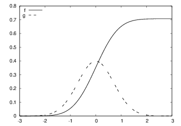
Figure 1 shows how the population stabilizes, i.e., that \( x_n \) approaches \( M \) as \( N \) becomes large (of the same magnitude as \( M \)).

If the equation stabilizes as \( n\rightarrow\infty \), it means that \( x_{n}=x_{n-1} \) in this limit. The equation then reduces to $$ \begin{equation*} x_n = x_{n} + {\varrho\over 100} x_{n}\left(1 - {x_{n}\over M}\right)\tp \end{equation*} $$ By inserting \( x_n=M \) we see that this solution fulfills the equation. The same solution technique (i.e., setting \( x_{n}=x_{n-1} \)) can be used to check if \( x_n \) in a difference equation approaches a limit or not.

Mathematical models like (12) are often easier to work with if we scale the variables. Basically, this means that we divide each variable by a characteristic size of that variable such that the value of the new variable is typically 1. In the present case we can scale \( x_n \) by \( M \) and introduce a new variable, $$ \begin{equation*} y_n = {x_n\over M}\tp\end{equation*} $$ Similarly, \( x_0 \) is replaced by \( y_0=x_0/M \). Inserting \( x_n = My_n \) in (12) and dividing by \( M \) gives $$ \begin{equation} y_n = y_{n-1} + q y_{n-1}\left(1 - y_{n-1}\right), \tag{13} \end{equation} $$ where \( q=\varrho /100 \) is introduced to save typing. Equation (13) is simpler than (12) in that the solution lies approximately between \( y_0 \) and 1 (values larger than 1 can occur, see Exercise 19: Demonstrate oscillatory solutions of the logistic equation), and there are only two dimensionless input parameters to care about: \( q \) and \( y_0 \). To solve (12) we need knowledge of three parameters: \( x_0 \), \( \varrho \), and \( M \).

Payback of a loan

A loan \( L \) is to be paid back over \( N \) months. The payback in a month consists of the fraction \( L/N \) plus the interest increase of the loan. Let the annual interest rate for the loan be \( p \) percent. The monthly interest rate is then \( \frac{p}{12} \). The value of the loan after month \( n \) is \( x_n \), and the change from \( x_{n-1} \) can be modeled as $$ \begin{align} x_n &= x_{n-1} + {p\over 12\cdot 100}x_{n-1} - \left({p\over 12\cdot 100}x_{n-1} + {L\over N}\right), \tag{14}\\ &= x_{n-1} - {L\over N}, \tag{15} \end{align} $$ for \( n=1,\ldots,N\nonumber \). The initial condition is \( x_0=L \). A major difference between (15) and (6) is that all terms in the latter are proportional to \( x_n \) or \( x_{n-1} \), while (15) also contains a constant term (\( L/N \)). We say that (6) is homogeneous and linear, while (15) is inhomogeneous (because of the constant term) and linear. The mathematical solution of inhomogeneous equations are more difficult to find than the solution of homogeneous equations, but in a program there is no big difference: we just add the extra term \( -L/N \) in the formula for the difference equation.

The solution of (15) is not particularly exciting (just use (15) repeatedly to derive the solution \( x_n=L-nL/N \)). What is more interesting, is what we pay each month, \( y_n \). We can keep track of both \( y_n \) and \( x_n \) in a variant of the previous model: $$ \begin{align} y_n &= {p\over 12\cdot 100}x_{n-1} + {L\over N}, \tag{16}\\ x_n &= x_{n-1} + {p\over 12\cdot 100}x_{n-1} - y_n\tp \tag{17} \end{align} $$ Equations (16)-(17) is a system of difference equations. In a computer code, we simply update \( y_n \) first, and then we update \( x_n \), inside a loop over \( n \). Exercise 4: Compute the development of a loan asks you to do this.

The integral as a difference equation

Suppose a function \( f(x) \) is defined as the integral $$ \begin{equation} f(x) = \int\limits_{a}^x g(t)dt\tp \tag{18} \end{equation} $$ Our aim is to evaluate \( f(x) \) at a set of points \( x_0=a < x_1 < \cdots < x_N \). The value \( f(x_n) \) for any \( 0\leq n\leq N \) can be obtained by using the Trapezoidal rule for integration: $$ \begin{equation} f(x_n) = \sum_{k=0}^{n-1} \frac{1}{2}(x_{k+1}-x_k)(g(x_k) + g(x_{k+1})), \tag{19} \end{equation} $$ which is nothing but the sum of the areas of the trapezoids up to the point \( x_n \). We realize that \( f(x_{n+1}) \) is the sum above plus the area of the next trapezoid: $$ \begin{equation} f(x_{n+1}) = f(x_n) + \frac{1}{2}(x_{n+1}-x_n)(g(x_n) + g(x_{n+1}))\tp \tag{20} \end{equation} $$ This is a much more efficient formula than using (19) with \( n \) replaced by \( n+1 \), since we do not need to recompute the areas of the first \( n \) trapezoids.

Formula (20) gives the idea of computing all the \( f(x_n) \) values through a difference equation. Define \( f_n \) as \( f(x_n) \) and consider \( x_0=a \), and \( x_1, \ldots,x_N \) as given. We know that \( f_0=0 \). Then $$ \begin{equation} f_n = f_{n-1} + \frac{1}{2}(x_{n}-x_{n-1})(g(x_{n-1}) + g(x_n)), \tag{21} \end{equation} $$ for \( n=1,2,\ldots,N \). By introducing \( g_n \) for \( g(x_n) \) as an extra variable in the difference equation, we can avoid recomputing \( g(x_n) \) when we compute \( f_{n+1} \): $$ \begin{align} g_n &= g(x_n), \tag{22}\\ f_n &= f_{n-1} + \frac{1}{2}(x_{n}-x_{n-1})(g_{n-1} + g_n), \tag{23} \end{align} $$ with initial conditions \( f_0=0 \) and \( g_0=g(a) \).

A function can take \( g \), \( a \), \( x \), and \( N \) as input and return arrays x and f for \( x_0,\ldots,x_N \) and the corresponding integral values \( f_0,\ldots,f_N \):

def integral(g, a, x, N=20):
    index_set = range(N+1)
    x = np.linspace(a, x, N+1)
    g_ = np.zeros_like(x)
    f = np.zeros_like(x)
    g_[0] = g(x[0])
    f[0] = 0

    for n in index_set[1:]:
        g_[n] = g(x[n])
        f[n] = f[n-1] + 0.5*(x[n] - x[n-1])*(g_[n-1] + g_[n])
    return x, f

Our first task, after having implemented a mathematical calculation, is to verify the result. Here we can make use of the nice fact that the Trapezoidal rule is exact for linear functions \( g(t) \):

def test_integral():
    def g_test(t):
        """Linear integrand."""
        return 2*t + 1

    def f_test(x, a):
        """Exact integral of g_test."""
        return x**2 + x - (a**2 + a)

    a = 2
    x, f = integral(g_test, a, x=10)
    f_exact = f_test(x, a)
    assert np.allclose(f_exact, f)

A realistic application is to apply the integral function to some \( g(t) \) where there is no formula for the analytical integral, e.g., $$ \begin{equation*} g(t) = \frac{1}{\sqrt{2\pi}}\exp{\left(-t^2\right)}\tp\end{equation*} $$ The code may look like

def demo():
    """Integrate the Gaussian function."""
    from numpy import sqrt, pi, exp

    def g(t):
        return 1./sqrt(2*pi)*exp(-t**2)

    t, f = integral(g, a=-3, x=3, N=200)
    integrand = g(t)
    from scitools.std import plot
    plot(t, f, 'r-',
         t, integrand, 'y-',
         legend=('f', 'g'),
         legend_loc='upper left',
         savefig='tmp.pdf')

Taylor series as a difference equation

Consider the following system of two difference equations $$ \begin{align} e_n &= e_{n-1} + a_{n-1}, \tag{24}\\ a_n &= {x\over n} a_{n-1}, \tag{25} \end{align} $$ with initial conditions \( e_0=0 \) and \( a_0=1 \). We can start to nest the solution: $$ \begin{align*} e_1 &= 0 + a_0 = 0 + 1 = 1,\\ a_1 &= x,\\ e_2 &= e_1 + a_1= 1+x,\\ a_2 &= {x\over2}a_1 = {x^2\over 2},\\ e_3 &= e_2 + a_2 = 1 + x + {x^2\over 2},\\ e_4 &= 1 + x + {x^2\over 2} + {x^3\over 3\cdot 2},\\ e_5 &= 1 + x + {x^2\over 2} + {x^3\over 3\cdot 2} + {x^4\over 4\cdot 3\cdot 2} \end{align*} $$ The observant reader who has heard about Taylor series will recognize this as the Taylor series of \( e^x \): $$ \begin{equation} e^x= \sum_{n=0}^\infty {x^n\over n!}\tp \tag{26} \end{equation} $$

How do we derive a system like (24)-(25) for computing the Taylor polynomial approximation to \( e^x \)? The starting point is the sum \( \sum_{n=0}^\infty {x^n\over n!} \). This sum is coded by adding new terms to an accumulation variable in a loop. The mathematical counterpart to this code is a difference equation $$ \begin{equation} e_{n+1} = e_{n} + {x^{n}\over {n}!},\quad e_{0}=0,\ n=0,1,2,\ldots\tp \tag{27} \end{equation} $$ or equivalently (just replace \( n \) by \( n-1 \)): $$ \begin{equation} e_n = e_{n-1} + {x^{n-1}\over {n-1}!},\quad e_{0}=0,\ n=1,2,3,\ldots\tp \tag{28} \end{equation} $$ Now comes the important observation: the term \( x^n/n! \) contains many of the computations we already performed for the previous term \( x^{n-1}/(n-1)! \) because $$ \begin{equation*} {x^{n}\over n!} = {x\cdot x \cdots x\over n(n-1)(n-2)\cdots 1},\quad {x^{n-1}\over (n-1)!} = {x\cdot x \cdots x\over (n-1)(n-2)(n-3)\cdots 1}\tp\end{equation*} $$ Let \( a_{n}=x^n/n! \). We see that we can go from \( a_{n-1} \) to \( a_{n} \) by multiplying \( a_{n-1} \) by \( x/n \): $$ \begin{equation} {x\over n}a_{n-1}={x\over n}{x^{n-1}\over (n-1)!} = {x^n\over n!} = a_{n}, \tag{29} \end{equation} $$ which is nothing but (25). We also realize that \( a_0=1 \) is the initial condition for this difference equation. In other words, (24) sums the Taylor polynomial, and (25) updates each term in the sum.

The system (24)-(25) is very easy to implement in a program and constitutes an efficient way to compute (26). The function exp_diffeq does the work:

def exp_diffeq(x, N):
    n = 1
    an_prev = 1.0  # a_0
    en_prev = 0.0  # e_0
    while n <= N:
        en = en_prev + an_prev
        an = x/n*an_prev
        en_prev = en
        an_prev = an
        n += 1
    return en

Making a living from a fortune

Suppose you want to live on a fortune \( F \). You have invested the money in a safe way that gives an annual interest of \( p \) percent. Every year you plan to consume an amount \( c_n \), where \( n \) counts years. The development of your fortune \( x_n \) from one year to the other can then be modeled by $$ \begin{equation} x_n = x_{n-1} + {p\over 100}x_{n-1} - c_{n-1},\quad x_0=F\tp \tag{30} \end{equation} $$ A simple example is to keep \( c \) constant, say \( q \) percent of the interest the first year: $$ \begin{equation} x_n = x_{n-1} + {p\over 100}x_{n-1} - {pq\over 10^4}F,\quad x_0=F\tp \tag{31} \end{equation} $$ A more realistic model is to assume some inflation of \( I \) percent per year. You will then like to increase \( c_n \) by the inflation. We can extend the model in two ways. The simplest and clearest way, in the author's opinion, is to track the evolution of two sequences \( x_n \) and \( c_n \): $$ \begin{align} x_n &= x_{n-1} + {p\over 100}x_{n-1} - c_{n-1},\quad x_0=F,\ c_0 = {pq\over 10^4}F, \tag{32}\\ c_n &= c_{n-1} + {I\over100}c_{n-1} \tp \tag{33} \end{align} $$ This is a system of two difference equations with two unknowns. The solution method is, nevertheless, not much more complicated than the method for a difference equation in one unknown, since we can first compute \( x_n \) from (32) and then update the \( c_n \) value from (33). You are encouraged to write the program (see Exercise 5: Solve a system of difference equations).

Another way of making a difference equation for the case with inflation, is to use an explicit formula for \( c_{n-1} \), i.e., solve (32) and end up with a formula like (4). Then we can insert the explicit formula $$ \begin{equation*} c_{n-1} = \left( 1 + {I\over 100}\right)^{n-1} {pq\over 10^4}F\end{equation*} $$ in (30), resulting in only one difference equation to solve.

Newton's method

The difference equation $$ \begin{equation} x_n = x_{n-1} - {f(x_{n-1})\over f'(x_{n-1})},\quad x_0 \hbox{ given}, \tag{34} \end{equation} $$ generates a sequence \( x_n \) where, if the sequence converges (i.e., if \( x_n - x_{n-1}\rightarrow 0 \)), \( x_n \) approaches a root of \( f(x) \). That is, \( x_n\rightarrow x \), where \( x \) solves the equation \( f(x)=0 \). Equation (34) is the famous Newton's method for solving nonlinear algebraic equations \( f(x)=0 \). When \( f(x) \) is not linear, i.e., \( f(x) \) is not on the form \( ax+b \) with constant \( a \) and \( b \), (34) becomes a nonlinear difference equation. This complicates analytical treatment of difference equations, but poses no extra difficulties for numerical solution.

We can quickly sketch the derivation of (34). Suppose we want to solve the equation $$ \begin{equation*} f(x)=0 \end{equation*} $$ and that we already have an approximate solution \( x_{n-1} \). If \( f(x) \) were linear, \( f(x)=ax+b \), it would be very easy to solve \( f(x)=0 \): \( x=-b/a \). The idea is therefore to approximate \( f(x) \) in the vicinity of \( x=x_{n-1} \) by a linear function, i.e., a straight line \( f(x)\approx \tilde f(x) = ax+b \). This line should have the same slope as \( f(x) \), i.e., \( a=f'(x_{n-1}) \), and both the line and \( f \) should have the same value at \( x=x_{n-1} \). From this condition one can find \( b=f(x_{n-1}) -x_{n-1}f'(x_{n-1}) \). The approximate function (line) is then $$ \begin{equation} \tilde f(x) = f(x_{n-1}) + f'(x_{n-1})(x-x_{n-1})\tp \tag{35} \end{equation} $$ This expression is just the two first terms of a Taylor series approximation to \( f(x) \) at \( x=x_{n-1} \). It is now easy to solve \( \tilde f(x)=0 \) with respect to \( x \), and we get $$ \begin{equation} x = x_{n-1} - {f(x_{n-1})\over f'(x_{n-1})}\tp \tag{36} \end{equation} $$ Since \( \tilde f \) is only an approximation to \( f \), \( x \) in (36) is only an approximation to a root of \( f(x)=0 \). Hopefully, the approximation is better than \( x_{n-1} \) so we set \( x_n=x \) as the next term in a sequence that we hope converges to the correct root. However, convergence depends highly on the shape of \( f(x) \), and there is no guarantee that the method will work.

The previous programs for solving difference equations have typically calculated a sequence \( x_n \) up to \( n=N \), where \( N \) is given. When using (34) to find roots of nonlinear equations, we do not know a suitable \( N \) in advance that leads to an \( x_n \) where \( f(x_n) \) is sufficiently close to zero. We therefore have to keep on increasing \( n \) until \( f(x_n) < \epsilon \) for some small \( \epsilon \). Of course, the sequence diverges, we will keep on forever, so there must be some maximum allowable limit on \( n \), which we may take as \( N \).

It can be convenient to have the solution of (34) as a function for easy reuse. Here is a first rough implementation:

def Newton(f, x, dfdx, epsilon=1.0E-7, N=100):
    n = 0
    while abs(f(x)) > epsilon and n <= N:
        x = x - f(x)/dfdx(x)
        n += 1
    return x, n, f(x)

Another, more serious, problem is the possibility dividing by zero. Almost as serious, is dividing by a very small number that creates a large value, which might cause Newton's method to diverge. Therefore, we should test for small values of \( f'(x) \) and write a warning or raise an exception.

Another improvement is to add a boolean argument store to indicate whether we want the \( (x,f(x)) \) values during the iterations to be stored in a list or not. These intermediate values can be handy if we want to print out or plot the convergence behavior of Newton's method.

An improved Newton function can now be coded as

def Newton(f, x, dfdx, epsilon=1.0E-7, N=100, store=False):
    f_value = f(x)
    n = 0
    if store: info = [(x, f_value)]
    while abs(f_value) > epsilon and n <= N:
        dfdx_value = float(dfdx(x))
        if abs(dfdx_value) < 1E-14:
            raise ValueError("Newton: f'(%g)=%g" % (x, dfdx_value))

        x = x - f_value/dfdx_value

        n += 1
        f_value = f(x)
        if store: info.append((x, f_value))
    if store:
        return x, info
    else:
        return x, n, f_value

Note that to use the Newton function, we need to calculate the derivative \( f'(x) \) and implement it as a Python function and provide it as the dfdx argument. Also note that what we return depends on whether we store \( (x,f(x)) \) information during the iterations or not.

It is quite common to test if dfdx(x) is zero in an implementation of Newton's method, but this is not strictly necessary in Python since an exception ZeroDivisionError is always raised when dividing by zero.

We can apply the Newton function to solve the equation \( e^{-0.1x^2}\sin (\frac{\pi}{2}x) =0 \):

from math import sin, cos, exp, pi
import sys
from Newton import Newton

def g(x):
    return exp(-0.1*x**2)*sin(pi/2*x)

def dg(x):
    return -2*0.1*x*exp(-0.1*x**2)*sin(pi/2*x) + \ 
           pi/2*exp(-0.1*x**2)*cos(pi/2*x)

x0 = float(sys.argv[1])
x, info = Newton(g, x0, dg, store=True)
print 'root:', x
for i in range(len(info)):
    print 'Iteration %3d: f(%g)=%g' % \ 
          (i, info[i][0], info[i][1])

root: 1.999999999768449
Iteration  0: f(1.7)=0.340044
Iteration  1: f(1.99215)=0.00828786
Iteration  2: f(1.99998)=2.53347e-05
Iteration  3: f(2)=2.43808e-10

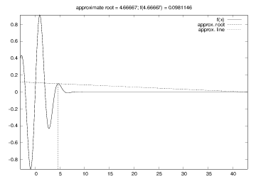
Trying a start value of 3, we would expect the method to find the root \( x=2 \) or \( x=4 \), but now we get

root: 42.49723316011362
Iteration  0: f(3)=-0.40657
Iteration  1: f(4.66667)=0.0981146
Iteration  2: f(42.4972)=-2.59037e-79

The demo program Newton_movie.py can be used to investigate the strange behavior. This program takes five command-line arguments: a formula for \( f(x) \), a formula for \( f'(x) \) (or the word numeric, which indicates a numerical approximation of \( f'(x) \)), a guess at the root, and the minimum and maximum \( x \) values in the plots. We try the following case with the program:

Newton_movie.py 'exp(-0.1*x**2)*sin(pi/2*x)' numeric 3 -3 43

You can run the Newton_movie.py program with other values of the initial root and observe that the method usually finds the nearest roots.

The inverse of a function

Given a function \( f(x) \), the inverse function of \( f \), say we call it \( g(x) \), has the property that if we apply \( g \) to the value \( f(x) \), we get \( x \) back: $$ \begin{equation*} g(f(x)) = x\tp\end{equation*} $$ Similarly, if we apply \( f \) to the value \( g(x) \), we get \( x \): $$ \begin{equation} f(g(x)) = x\tp \tag{37} \end{equation} $$ By hand, you substitute \( g(x) \) by (say) \( y \) in (37) and solve (37) with respect to \( y \) to find some \( x \) expression for the inverse function. For example, given \( f(x)=x^2-1 \), we must solve \( y^2 - 1 = x \) with respect to \( y \). To ensure a unique solution for \( y \), the \( x \) values have to be limited to an interval where \( f(x) \) is monotone, say \( x\in [0,1] \) in the present example. Solving for \( y \) gives \( y = \sqrt{1+x} \), therefore \( g(x) = \sqrt{1+x} \). It is easy to check that \( f(g(x)) = (\sqrt{1+x})^2 - 1 = x \).

Numerically, we can use the "definition" (37) of the inverse function \( g \) at one point at a time. Suppose we have a sequence of points \( x_0 < x_1 < \cdots < x_{N} \) along the \( x \) axis such that \( f \) is monotone in \( [x_0,x_N] \): \( f(x_0)>f(x_1)>\cdots >f(x_N) \) or \( f(x_0) < f(x_1) < \cdots < f(x_N) \). For each point \( x_i \), we have $$ \begin{equation*} f(g(x_i)) = x_i\tp \end{equation*} $$ The value \( g(x_i) \) is unknown, so let us call it \( \gamma \). The equation $$ \begin{equation} f(\gamma) = x_i \tag{38} \end{equation} $$ can be solved be respect \( \gamma \). However, (38) is in general nonlinear if \( f \) is a nonlinear function of \( x \). We must then use, e.g., Newton's method to solve (38). Newton's method works for an equation phrased as \( f(x)=0 \), which in our case is \( f(\gamma )-x_i=0 \), i.e., we seek the roots of the function \( F(\gamma) \equiv f(\gamma) - x_i \). Also the derivative \( F'(\gamma) \) is needed in Newton's method. For simplicity we may use an approximate finite difference: $$ \begin{equation*} {dF\over d\gamma} \approx {F(\gamma + h) - F(\gamma - h)\over 2h}\tp \end{equation*} $$ As start value \( \gamma_0 \), we can use the previously computed \( g \) value: \( g_{i-1} \). We introduce the short notation \( \gamma = \hbox{Newton}(F, \gamma_0) \) to indicate the solution of \( F(\gamma)=0 \) with initial guess \( \gamma_0 \).

The computation of all the \( g_0,\ldots,g_N \) values can now be expressed by $$ \begin{equation} g_i = \hbox{Newton}(F, g_{i-1}),\quad i=1,\ldots,N, \tag{39} \end{equation} $$ and for the first point we may use \( x_0 \) as start value (for instance): $$ \begin{equation} g_0 = \hbox{Newton}(F, x_0)\tp \tag{40} \end{equation} $$ Equations (39)-(40) constitute a difference equation for \( g_i \), since given \( g_{i-1} \), we can compute the next element of the sequence by (39). Because (39) is a nonlinear equation in the new value \( g_i \), and (39) is therefore an example of a nonlinear difference equation.

The following program computes the inverse function \( g(x) \) of \( f(x) \) at some discrete points \( x_0,\ldots,x_N \). Our sample function is \( f(x)=x^2-1 \):

from Newton import Newton
from scitools.std import *

def f(x):
    return x**2 - 1

def F(gamma):
    return f(gamma) - xi

def dFdx(gamma):
    return (F(gamma+h) - F(gamma-h))/(2*h)

h = 1E-6
x = linspace(0.01, 3, 21)
g = zeros(len(x))

for i in range(len(x)):
    xi = x[i]

    # Compute start value (use last g[i-1] if possible)
    if i == 0:
        gamma0 = x[0]
    else:
        gamma0 = g[i-1]

    gamma, n, F_value = Newton(F, gamma0, dFdx)
    g[i] = gamma

plot(x, f(x), 'r-', x, g, 'b-',
     title='f1', legend=('original', 'inverse'))

« Previous

Next »