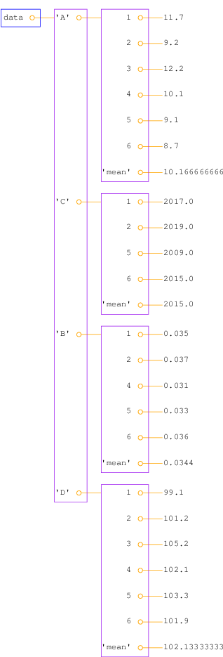
Figure 1: Illustration of the nested dictionary created in the table2dict.py program.
This chapter is taken from the book A Primer on Scientific Programming with Python by H. P. Langtangen, 5th edition, Springer, 2016.
So far in the document we have stored information in various types of objects, such as numbers, strings, list, and arrays. A dictionary is a very flexible object for storing various kind of information, and in particular when reading files. It is therefore time to introduce the popular dictionary type.
A list is a collection of objects indexed by an integer going from 0 to the number of elements minus one. Instead of looking up an element through an integer index, it can be more handy to use a text. Roughly speaking, a list where the index can be a text is called a {dictionary} in Python. Other computer languages use other names for the same thing: HashMap, hash, associative array, or map.
Suppose we need to store the temperatures from three cities: Oslo, London, and Paris. For this purpose we can use a list,
temps = [13, 15.4, 17.5]
temps[1].
A dictionary with the city name as index is more convenient, because
this allows us to write temps['London'] to look up the temperature
in London. Such a dictionary is created by one of the following two statements
temps = {'Oslo': 13, 'London': 15.4, 'Paris': 17.5}
# or
temps = dict(Oslo=13, London=15.4, Paris=17.5)
temps['Madrid'] = 26.0
temps dictionary has now four text-value pairs, and
a print temps yields
{'Oslo': 13, 'London': 15.4, 'Paris': 17.5, 'Madrid': 26.0}
The string "indices" in a dictionary are called keys.
To loop over the keys in a dictionary d, one writes
for key in d: and works with key and the
corresponding value d[key]
inside the loop. We may apply this technique to write out the
temperatures in the temps dictionary from the previous paragraph:
>>> for city in temps:
...     print 'The temperature in %s is %g' % (city, temps[city])
...
The temperature in Paris is 17.5
The temperature in Oslo is 13
The temperature in London is 15.4
The temperature in Madrid is 26
if key in d:
>>> if 'Berlin' in temps:
...     print 'Berlin:', temps['Berlin']
... else:
...     print 'No temperature data for Berlin'
...
No temperature data for Berlin
key in d yields a standard boolean expression, e.g.,
>>> 'Oslo' in temps
True
>>> temps.keys()
['Paris', 'Oslo', 'London', 'Madrid']
>>> temps.values()
[17.5, 13, 15.4, 26.0]
keys method in dictionaries
is that the order of the returned list of
keys is unpredictable. If you need to traverse the keys in a certain
order, you can sort the keys. A loop over the keys in the
temps dictionary in alphabetic order is written as
>>> for city in sorted(temps):
...     print city
...
London
Madrid
Oslo
Paris
OrderedDict
where the key-value pairs has a specific order, see
the section Dictionaries with default values and ordering.
A key-value pair can be removed by del d[key]:
>>> del temps['Oslo']
>>> temps
{'Paris': 17.5, 'London': 15.4, 'Madrid': 26.0}
>>> len(temps)  # no of key-value pairs in dictionary
3
Sometimes we need to take a copy of a dictionary:
>>> temps_copy = temps.copy()
>>> del temps_copy['Paris']   # this does not affect temps
>>> temps_copy
{'London': 15.4, 'Madrid': 26.0}
>>> temps
{'Paris': 17.5, 'London': 15.4, 'Madrid': 26.0}
>>> t1 = temps
>>> t1['Stockholm'] = 10.0    # change t1
>>> temps                     # temps is also changed
{'Stockholm': 10.0, 'Paris': 17.5, 'London': 15.4, 'Madrid': 26.0}
temps is affected by adding a new key-value pair
to t1, t1 must be a copy of temps.
In Python version 2.x, temps.keys() returns a list object while
in Python version 3.x, temps.keys() only enables iterating over
the keys. To write code that works with both versions one can
use list(temps.keys()) in the cases where a list is really
needed and just temps.keys() in a for loop over the keys.
Python objects that cannot change their contents
are known as immutable data types
and consist of int, float, complex,
str, and tuple. Lists and dictionaries
can change their contents and are called
mutable objects.
The keys in a dictionary are not restricted to be strings. In fact, any immutable Python object can be used as key. For example, if you want a list as key, it cannot be used since lists can change their contents are hence mutable objects, but a tuple will do, since it is immutable.
A common type of key in dictionaries is integers. Next we shall explain how dictionaries with integers as key provide a handy way of representing polynomials. Consider the polynomial $$ \begin{equation*} p(x)=-1 + x^2 + 3x^7\tp \end{equation*} $$ The data associated with this polynomial can be viewed as a set of power-coefficient pairs, in this case the coefficient \( -1 \) belongs to power 0, the coefficient 1 belongs to power 2, and the coefficient 3 belongs to power 7. A dictionary can be used to map a power to a coefficient:
p = {0: -1, 2: 1, 7: 3}
p = [-1, 0, 1, 0, 0, 0, 0, 3]
The following function can be used to evaluate a polynomial represented as a dictionary:
def eval_poly_dict(poly, x):
    sum = 0.0
    for power in poly:
        sum += poly[power]*x**power
    return sum
poly argument must be a dictionary where poly[power]
holds the coefficient associated with the term x**power.
A more compact implementation can make use of Python's sum
function to sum the elements of a list:
def eval_poly_dict2(poly, x):
    return sum([poly[power]*x**power for power in poly])
sum
function. We can in fact drop the brackets and storing all the
poly[power]*x**power numbers in a list, because
sum can directly add elements of an iterator (like for power in poly):
def eval_poly_dict2(poly, x):
    return sum(poly[power]*x**power for power in poly)
The name sum appears in both eval_poly_dict and eval_poly_dict2.
In the former, sum is a float object, and in the
latter, sum is a built-in Python function. When we set sum=0.0 in the first
implementation, we bind the name sum to a new float object, and
the built-in Python function associated with the name sum is then no
longer accessible inside the eval_poly_dict function. (Actually, this is not
strictly correct, because sum is a local variable while the
built-in Python sum function is associated with a global name sum,
which can always be reached through globals()['sum'].)
Outside the eval_poly_dict function,
nevertheless, sum will be Python's summation function and the local
sum variable inside the eval_poly_dict function is destroyed.
As a rule of thumb, avoid using sum or other names associated with frequently
used functions as new variables unless you are in a very small function
(like eval_poly_dict) where there is no danger that you need
the original meaning of the name.
With a list instead of dictionary for representing the polynomial, a slightly different evaluation function is needed:
def eval_poly_list(poly, x):
    sum = 0
    for power in range(len(poly)):
        sum += poly[power]*x**power
    return sum
poly list, eval_poly_list must
perform all the multiplications with the zeros, while eval_poly_dict
computes with the non-zero coefficients only and is hence more
efficient.
Another major advantage of using a dictionary to represent a polynomial rather than a list is that negative powers are easily allowed, e.g.,
p = {-3: 0.5, 4: 2}
p = [0.5, 0, 0, 0, 0, 0, 0, 2]
p[i] is the coefficient associated with the
power i-3. In particular, the eval_poly_list function will no longer
work for such lists, while the eval_poly_dict function
works also for dictionaries with negative keys (powers).
There is a dictionary counterpart to list comprehensions, called
dictionary comprehensions, for quickly generating parameterized
key-value pairs
with a for loop. Such a construction is convenient to generate
the coefficients in a polynomial:
from math import factorial
d = {k: (-1)**k/float(factorial(k)) for k in range(n+1)}
d dictionary now contains the power-coefficient pairs of the
Taylor polynomial of degree n for \( e^{-x} \). (Note the use of float
to avoid integer division.)
You are now encouraged to solve Exercise 11: Compute the derivative of a polynomial to become more familiar with the concept of dictionaries.
Looking up keys that are not present in the dictionary requires special treatment. Consider a polynomial dictionary of the type introduced in the section Example: Polynomials as dictionaries. Say we have \( 2x^{-3} -1.5x^{-1} -2x^2 \) represented by
p1 = {-3: 2, -1: -1.5, 2: -2}
p1[1],
this operation results in a KeyError since 1 is
not a registered key in p1. We therefore need to do either
if key in p1:
   value = p1[key]
value = p1.get(key, 0.0)
p1.get returns p1[key] if key in p1
and the default value 0.0 if not.
A third possibility is to work with a dictionary with a
default value:
from collections import defaultdict

def polynomial_coeff_default():
    # default value for polynomial dictionary
    return 0.0

p2 = defaultdict(polynomial_coeff_default)
p2.update(p1)
p2 can be indexed by any key, and for unregistered keys
the polynomial_coeff_default function is called to provide
a value. This must be a function without arguments. Usually,
a separate function is never made, but either a type is inserted
or a lambda function. The example above is equivalent to
p2 = defaultdict(lambda: 0.0)
p2 = defaultdict(float)
float() is called for each unknown key,
and float() returns a float object with zero value.
Now we can look up p2[1] and get the default value 0.
It must be remarked that this key is then a part of the dictionary:
>>> p2 = defaultdict(lambda: 0.0)
>>> p2.update({2: 8})  # only one key
>>> p2[1]
0.0
>>> p2[0]
0.0
>>> p2[-2]
0.0
>>> print p2
{0: 0.0, 1: 0.0, 2: 8, -2: 0.0}
The elements of a dictionary have an undefined order. For example,
>>> p1 = {-3: 2, -1: -1.5, 2: -2}
>>> print p1
{2: -2, -3: 2, -1: -1.5}
>>> for key in sorted(p1):
...     print key, p1[key]
...
-3 2
-1 -1.5
2 -2
sorted function also accept an optional argument where
the user can supply a function that sorts two
keys.
However, Python features a dictionary type that preserves the order of the keys as they were registered:
>>> from collections import OrderedDict
>>> p2 = OrderedDict({-3: 2, -1: -1.5, 2: -2})
>>> print p2
OrderedDict([(2, -2), (-3, 2), (-1, -1.5)])
>>> p2[-5] = 6
>>> for key in p2:
...     print key, p2[key]
...
2 -2
-3 2
-1 -1.5
-5 6
Here is an example with dates as keys where the order is important.
>>> data = {'Jan 2': 33, 'Jan 16': 0.1, 'Feb 2': 2}
>>> for date in data:
...     print date, data[date]
...
Feb 2 2
Jan 2 33
Jan 16 0.1
OrderedDict
>>> data = OrderedDict()
>>> data['Jan 2'] = 33
>>> data['Jan 16'] = 0.1
>>> data['Feb 2'] = 2
>>> for date in data:
...     print date, data[date]
...
Jan2 33
Jan 16 0.1
Feb 2 2
A comment on alternative solutions
should be made here. Trying to sort the data dictionary
when it is an ordinary dict object does not help, as by
default the sorting will be alphabetically, resulting in
the sequence 'Feb 2', 'Jan 16', and 'Jan 2'.
What does help, however, is to use Python's datetime objects
as keys reflecting dates, since these objects will be correctly
sorted. A datetime object can be created from
a string like 'Jan 2, 2017' using a special syntax
(see the module documentation). The relevant code is
>>> import datetime
>>> data = {}
>>> d = datetime.datetime.strptime  # short form
>>> data[d('Jan 2, 2017', '%b %d, %Y')] = 33
>>> data[d('Jan 16, 2017', '%b %d, %Y')] = 0.1
>>> data[d('Feb 2, 2017', '%b %d, %Y')] = 2
>>> for date in sorted(data):
...     print date, data[date]
...
2017-01-02 00:00:00 33
2017-01-16 00:00:00 0.1
2017-02-02 00:00:00 2
datetime object and set to
00:00:00 when not specified.
While OrderedDict provides a simpler and shorter solution
to keeping keys (here dates) in the right order in a dictionary,
using datetime objects for dates has many advantages: dates can be
formatted and written out in various ways, counting days between two dates is
easy,
calculating the corresponding week number and name of the weekday
is supported, to mention some functionality.
The file files/densities.dat contains a table of densities of
various substances measured in \( \hbox{g}/\hbox{cm}^3 \):
air         0.0012
gasoline    0.67
ice         0.9
pure water  1.0
seawater    1.025
human body  1.03
limestone   2.6
granite     2.7
iron        7.8
silver      10.5
mercury     13.6
gold        18.9
platinium   21.4
Earth mean  5.52
Earth core  13
Moon        3.3
Sun mean    1.4
Sun core    160
proton      2.3E+14
In a program we want to access these density data. A dictionary with the name of the substance as key and the corresponding density as value seems well suited for storing the data.
We can read the densities.dat file line by line, split each line
into words, use a float conversion of the last word as density value,
and the remaining one or two words as key in the dictionary.
def read_densities(filename):
    infile = open(filename, 'r')
    densities = {}
    for line in infile:
        words = line.split()
        density = float(words[-1])

        if len(words[:-1]) == 2:
            substance = words[0] + ' ' + words[1]
        else:
            substance = words[0]

        densities[substance] = density
    infile.close()
    return densities

densities = read_densities('densities.dat')
We are given a data file with measurements of some properties
with given names (here A, B, C ...).
Each property is measured a given number of times.
The data are organized as a table where the rows contain
the measurements and the columns represent the measured properties:
       A        B       C      D
1     11.7    0.035    2017    99.1
2      9.2    0.037    2019   101.2
3     12.2     no       no    105.2
4     10.1    0.031     no    102.1
5      9.1    0.033    2009   103.3
6      8.7    0.036    2015   101.9
The word no stands for no data, i.e., we lack a measurement.
We want to read this table into a dictionary data so that
we can look up measurement no. i of (say) property C
as data['C'][i].
For each property p, we want to compute the mean of all measurements
and store this as data[p]['mean'].
The algorithm for creating the data dictionary goes as follows:
examine the first line: split it into words and
initialize a dictionary with the property names
as keys and empty dictionaries {} as values

for each of the remaining lines in the file:
    split the line into words
    for each word after the first:
        if the word is not `no`:
            transform the word to a real number and store
            the number in the relevant dictionary
no:A new aspect needed in the solution is nested dictionaries, that is, dictionaries of dictionaries. The latter topic is first explained, via an example:
>>> d = {'key1': {'key1': 2, 'key2': 3}, 'key2': 7}
d['key1'] is a dictionary, which we can index with its
keys key1 and key2:
>>> d['key1']            # this is a dictionary
{'key2': 3, 'key1': 2}
>>> type(d['key1'])      # proof
<type 'dict'>
>>> d['key1']['key1']    # index a nested dictionary
2
>>> d['key1']['key2']
3
d['key2']
since that value is just an integer:
>>> d['key2']['key1']
  ...
TypeError: unsubscriptable object
>>> type(d['key2'])
<type 'int'>
When we have understood the concept of
nested dictionaries, we are in a position
to present a complete code that solves our problem
of loading the tabular data in the file table.dat into a nested
dictionary data and computing mean values.
First, we list the program, stored in the file
table2dict.py,
and display the program's output. Thereafter, we dissect the code
in detail.
infile = open('table.dat', 'r')
lines = infile.readlines()
infile.close()
data = {}   #  data[property][measurement_no] = propertyvalue
first_line = lines[0]
properties = first_line.split()
for p in properties:
    data[p] = {}

for line in lines[1:]:
    words = line.split()
    i = int(words[0])       # measurement number
    values = words[1:]      # values of properties
    for p, v in zip(properties, values):
        if v != 'no':
            data[p][i] = float(v)

# Compute mean values
for p in data:
    values = data[p].values()
    data[p]['mean'] = sum(values)/len(values)

for p in sorted(data):
    print 'Mean value of property %s = %g' % (p, data[p]['mean'])
Mean value of property A = 10.1667
Mean value of property B = 0.0344
Mean value of property C = 2015
Mean value of property D = 102.133
data dictionary, we may insert
import scitools.pprint2; scitools.pprint2.pprint(data)
{'A': {1: 11.7, 2: 9.2, 3: 12.2, 4: 10.1, 5: 9.1, 6: 8.7,
       'mean': 10.1667},
 'B': {1: 0.035, 2: 0.037, 4: 0.031, 5: 0.033, 6: 0.036,
       'mean': 0.0344},
 'C': {1: 2017, 2: 2019, 5: 2009, 6: 2015, 'mean': 2015},
 'D': {1: 99.1,
       2: 101.2,
       3: 105.2,
       4: 102.1,
       5: 103.3,
       6: 101.9,
       'mean': 102.133}}
To understand a computer program, you need to understand what the result of every statement is. Let us work through the code, almost line by line, and see what it does.
First, we load all the lines of the file into a list of strings
called lines.
The first_line variable refers to the string
' A B C D'
properties,
which then contains
['A', 'B', 'C', 'D']
for p in properties:
    data[p] = {}
for loop picks out the string
'1 11.7 0.035 2017 99.1'
line variable. We split this line into words,
the first word (words[0]) is the measurement number, while the
rest words[1:] is a list of property values, here named values.
To pair up the right properties and values, we loop over
the properties and values lists simultaneously:
    for p, v in zip(properties, values):
        if v != 'no':
            data[p][i] = float(v)
None).
Because the values list contains strings (words) read from
the file, we need to explicitly transform each string to a float number
before we can compute with the values.
Figure 1: Illustration of the nested dictionary created in the table2dict.py program.
After the for line in lines[1:] loop, we have a dictionary data of
dictionaries where all the property values are stored for each
measurement number and property name. Figure 1
shows a graphical representation of the data dictionary.
It remains to compute the average values. For each property name p,
i.e., key in the data dictionary, we can extract the recorded values
as the list data[p].values() and simply send this list to Python's
sum function and divide by the number of measured values for this
property, i.e., the length of the list:
for p in data:
    values = data[p].values()
    data[p]['mean'] = sum(values)/len(values)
for p in data:
    sum_values = 0
    for value in data[p]:
        sum_values += value
    data[p]['mean'] = sum_values/len(data[p])
When we want to look up a measurement no. n of property B, we
must recall that this particular measurement may be missing so we
must do a test if n is key in the dictionary data[p]:
if n in data['B']:
    value = data['B'][n]

# alternative:
value = data['B'][n] if n in data['B'] else None
We want to compare the evolution of the stock prices of some giant companies in the computer industry: Microsoft, Apple, and Google. Relevant data files for stock prices can be downloaded from http://finance.yahoo.com. Fill in the company's name and click on Search Finance in the top bar of this page and choose Historical Prices in the left pane. On the resulting web page one can specify start and end dates for the historical prices of the stock. The default values were used in this example. Ticking off Monthly values and clicking Get Prices result in a table of stock prices for each month since the stock was introduced. The table can be downloaded as a spreadsheet file in CSV format, typically looking like
Date,Open,High,Low,Close,Volume,Adj Close
2014-02-03,502.61,551.19,499.30,545.99,12244400,545.99
2014-01-02,555.68,560.20,493.55,500.60,15698500,497.62
2013-12-02,558.00,575.14,538.80,561.02,12382100,557.68
2013-11-01,524.02,558.33,512.38,556.07,9898700,552.76
2013-10-01,478.45,539.25,478.28,522.70,12598400,516.57
...
1984-11-01,25.00,26.50,21.87,24.75,5935500,2.71
1984-10-01,25.00,27.37,22.50,24.87,5654600,2.73
1984-09-07,26.50,29.00,24.62,25.12,5328800,2.76
stockprices_X.csv, where X is
Microsoft, Apple, or Google.
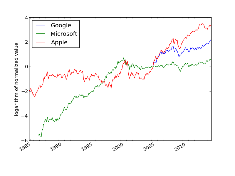
The task is visually illustrate the historical, relative stock market value of these companies. For this purpose it is natural to scale the prices of a company's stock to start at a unit value when the most recent company entered the market. Since the date of entry varies, the oldest data point can be skipped such that all data points correspond to the first trade day every month.
There are two major parts of this problem: reading the file and plotting the data. The reading part is quite straightforward, while the plotting part needs some special considerations since the \( x \) values in the plot are dates and not real numbers. In the forthcoming text we solve the individual subproblems one by one, showing the relevant Python snippets. The complete program is found in the file stockprices.py.
We start with the reading part. Since the reading will be repeated for
several companies, we create a function for extracting the relevant
data for a specific company. These data cover the dates in column 1
and the stock prices in the last column. Since we want to plot
prices versus dates, it will be convenient to turn the dates into
date objects. In more detail the algorithms has the following
points:
date (or datetime) objects goes as
from datetime import datetime
datefmt = '%Y-%m-%d'  # date format YYYY-MM-DD used in datetime
strdate = '2008-02-04'
datetime_object = datetime.strptime(strdate, datefmt)
date_object = datetime_object.date()
date and datetime object is that we
can compute with them and in particular used them in
plotting with Matplotlib.
We can now translate the algorithm to Python code:
from datetime import datetime

def read_file(filename):
    infile = open(filename, 'r')
    infile.readline()  # read column headings
    dates = [];  prices = []
    for line in infile:
        words = line.split(',')
        dates.append(words[0])
        prices.append(float(words[-1]))
    infile.close()
    dates.reverse()
    prices.reverse()
    # Convert dates on the form 'YYYY-MM-DD' to date objects
    datefmt = '%Y-%m-%d'
    dates = [datetime.strptime(_date, datefmt).date()
             for _date in dates]
    prices = np.array(prices)
    return dates[1:], prices[1:]
Although we work with three companies in this example, it is easy
and almost always a good idea to generalize the program to an
arbitrary number of companies. All we assume is that their
stock prices are in files with names of the form stockprices_X.csv,
where X is the company name.
With aid of the function call glob.glob('stockprices_*.csv')
we get a list of all such files. By looping over this list, extracting
the company name, and calling read_file, we can store the
dates and corresponding prices in dictionaries dates and prices,
indexed by the company name:
dates = {};  prices = {}
import glob, numpy as np
filenames = glob.glob('stockprices_*.csv')
companies = []
for filename in filenames:
    company = filename[12:-4]
    d, p = read_file(filename)
    dates[company] = d
    prices[company] = p
The next step is to normalize the prices such that they coincide
on a certain date. We pick this date as the first month we have
data for the youngest company. In lists of date or datetime
objects, we can use Python's max and min functions to extract
the newest and oldest date.
first_months = [dates[company][0] for company in dates]
normalize_date = max(first_months)
for company in dates:
    index = dates[company].index(normalize_date)
    prices[company] /= prices[company][index]

# Plot log of price versus years

import matplotlib.pyplot as plt
from matplotlib.dates import YearLocator, MonthLocator, DateFormatter

fig, ax = plt.subplots()
legends = []
for company in prices:
    ax.plot_date(dates[company], np.log(prices[company]),
                 '-', label=company)
    legends.append(company)
ax.legend(legends, loc='upper left')
ax.set_ylabel('logarithm of normalized value')

# Format the ticks
years    = YearLocator(5)   # major ticks every 5 years
months   = MonthLocator(6)  # minor ticks every 6 months
yearsfmt = DateFormatter('%Y')
ax.xaxis.set_major_locator(years)
ax.xaxis.set_major_formatter(yearsfmt)
ax.xaxis.set_minor_locator(months)
ax.autoscale_view()
fig.autofmt_xdate()

plt.savefig('tmp.pdf'); plt.savefig('tmp.png')
plt.show()
The normalized prices vary a lot, so to see the development over 30 years better, we decide to take the logarithm of the prices. The plotting procedure is somewhat involved so the reader should take the coming code more as a recipe than as a sequence of statement to really understand:
import matplotlib.pyplot as plt
from matplotlib.dates import YearLocator, MonthLocator, DateFormatter

fig, ax = plt.subplots()
legends = []
for company in prices:
    ax.plot_date(dates[company], np.log(prices[company]),
                 '-', label=company)
    legends.append(company)
ax.legend(legends, loc='upper left')
ax.set_ylabel('logarithm of normalized value')

# Format the ticks
years    = YearLocator(5)   # major ticks every 5 years
months   = MonthLocator(6)  # minor ticks every 6 months
yearsfmt = DateFormatter('%Y')
ax.xaxis.set_major_locator(years)
ax.xaxis.set_major_formatter(yearsfmt)
ax.xaxis.set_minor_locator(months)
ax.autoscale_view()
fig.autofmt_xdate()

plt.savefig('tmp.pdf'); plt.savefig('tmp.png')
Figure 2: The evolution of stock prices for three companies.