Figure 2: Plot of \( y = 10^5(x-0.9)^2(x-1.1)^3 \).
This chapter is taken from the book A Primer on Scientific Programming with Python by H. P. Langtangen, 5th edition, Springer, 2016.
Some class methods have names starting and ending with a double
underscore. These methods allow a special syntax in the program and
are called special methods. The constructor __init__ is one
example. This method is automatically called when an instance is
created (by calling the class as a function), but we do not need to
explicitly write __init__. Other special methods make it possible
to perform arithmetic operations with instances, to compare instances
with >, >=, !=, etc., to call instances as we call ordinary
functions, and to test if an instance evaluates to True or False,
to mention some possibilities.
Computing the value of the mathematical function represented by class
Y from the section Representing a function as a class, with y as the name of the
instance, is performed by writing y.value(t). If we could write
just y(t), the y instance would look as an ordinary function. Such
a syntax is indeed possible and offered by the special method named
__call__. Writing y(t) implies a call
y.__call__(t)
Y has the method __call__ defined.
We may easily add this special method:
class Y(object):
    ...
    def __call__(self, t):
        return self.v0*t - 0.5*self.g*t**2
value method is now redundant. A good programming
convention is to include a __call__ method in all classes that
represent a mathematical function. Instances with __call__ methods
are said to be callable objects, just as plain functions are
callable objects as well. The call syntax for callable objects is the
same, regardless of whether the object is a function or a class
instance. Given an object a,
if callable(a):
a behaves as a callable, i.e., if a
is a Python function or an instance with a __call__
method.
In particular, an instance of class Y can be passed as the
f argument to the diff function from the section Challenge: functions with parameters:
y = Y(v0=5)
dydt = diff(y, 0.1)
diff, we can test that f is not a function but an
instance of class Y. However, we only use f in calls, like
f(x), and for this purpose an instance with a
__call__ method works as a plain function.
This feature is very convenient.
The next section demonstrates a neat application of the call
operator __call__ in a numerical algorithm.
Given a Python implementation f(x) of a mathematical function
\( f(x) \), we want to create an object that behaves as a Python function
for computing the derivative \( f'(x) \). For example, if this object is
of type Derivative, we should be able to write something like
>>> def f(x):
        return x**3
...
>>> dfdx = Derivative(f)
>>> x = 2
>>> dfdx(x)
12.000000992884452
dfdx behaves as a straight Python function for implementing
the derivative \( 3x^2 \) of \( x^3 \) (well, the answer is only approximate,
with an error in the 7th decimal,
but the approximation can easily be improved).
Maple, Mathematica, and many other software packages can do exact
symbolic mathematics, including differentiation and integration. The
Python package sympy for symbolic mathematics
makes it trivial to calculate the exact derivative of
a large class of functions \( f(x) \) and turn the result into
an ordinary Python function. However, mathematical functions that are defined
in an algorithmic way (e.g., solution of another mathematical
problem), or functions with branches, random numbers, etc., pose
fundamental problems to symbolic differentiation, and then numerical
differentiation is required. Therefore we base the computation of
derivatives in Derivative instances on finite difference
formulas. Use of exact symbolic differentiation via SymPy is also possible.
The most basic (but not the best) formula for a numerical derivative is
$$
\begin{equation}
f'(x)\approx {f(x+h)-f(x)\over h}\tp
\tag{2}
\end{equation}
$$
The idea is that we make a class to hold the function to be
differentiated, call it f, and a step size h to be used in
(2).
These variables can be set in the
constructor. The __call__ operator computes the derivative with aid
of (1). All this can be
coded in a few lines:
class Derivative(object):
    def __init__(self, f, h=1E-5):
        self.f = f
        self.h = float(h)

    def __call__(self, x):
        f, h = self.f, self.h      # make short forms
        return (f(x+h) - f(x))/h
h into a float to avoid
potential integer division.
Below follows an application of the class to differentiate two functions \( f(x)=\sin x \) and \( g(t)=t^3 \):
>>> from math import sin, cos, pi
>>> df = Derivative(sin)
>>> x = pi
>>> df(x)
-1.000000082740371
>>> cos(x)  # exact
-1.0
>>> def g(t):
...     return t**3
...
>>> dg = Derivative(g)
>>> t = 1
>>> dg(t)  # compare with 3 (exact)
3.000000248221113
df(x) and dg(t)
look as ordinary Python functions that
evaluate the derivative of the functions sin(x) and g(t).
Class Derivative works for (almost) any function \( f(x) \).
It is a good programming habit to include a test function for verifying the implementation of a class. We can construct a test based on the fact that the approximate differentiation formula (2) is exact for linear functions:
def test_Derivative():
    # The formula is exact for linear functions, regardless of h
    f = lambda x: a*x + b
    a = 3.5; b = 8
    dfdx = Derivative(f, h=0.5)
    diff = abs(dfdx(4.5) - a)
    assert diff < 1E-14, 'bug in class Derivative, diff=%s' % diff
f. The alternative would be to define f in the standard way
def f(x):
    return a*x + b
f is that it remembers the variables a and
b when f is sent to class Derivative (it is a closure,
see the section Closures).
Note that the test function above follows
the conventions for test functions
outlined in the section A circle.
In what situations will it be convenient to automatically produce a
Python function df(x) which is the derivative of another Python
function f(x)? One example arises when solving nonlinear algebraic
equations \( f(x)=0 \) with Newton's method and we, because of laziness,
lack of time, or lack of training do not manage to derive \( f'(x) \) by
hand. Consider a function Newton for solving \( f(x)=0 \): Newton(f, x,
dfdx, epsilon=1.0E-7, N=100).
A specific implementation is found in the module file
Newton.py. The arguments are a
Python function f for \( f(x) \), a float x for the initial guess
(start value) of \( x \), a Python function dfdx for \( f'(x) \), a float
epsilon for the accuracy \( \epsilon \) of the root: the algorithms
iterates until \( |f(x)| < \epsilon \), and an int N for the maximum
number of iterations that we allow. All arguments are easy to
provide, except dfdx, which requires computing \( f'(x) \) by hand then
implementation of the formula in a Python function. Suppose our
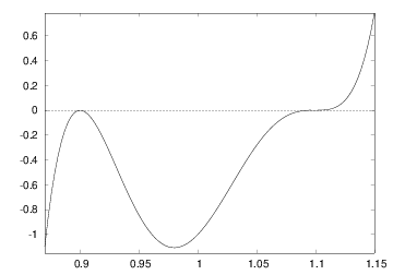
target equation reads
$$
\begin{equation*}
f(x) = 10^5(x-0.9)^2(x-1.1)^3=0 \thinspace .
\end{equation*}
$$
The function \( f(x) \) is plotted in Figure
2. The following session employs the
Derivative class to quickly make a derivative so we can call
Newton's method:
>>> from classes import Derivative
>>> from Newton import Newton
>>> def f(x):
...     return 100000*(x - 0.9)**2 * (x - 1.1)**3
...
>>> df = Derivative(f)
>>> Newton(f, 1.01, df, epsilon=1E-5)
(1.0987610068093443, 8, -7.5139644257961411e-06)
Figure 2: Plot of \( y = 10^5(x-0.9)^2(x-1.1)^3 \).
The exact root is 1.1, and the convergence toward this value is very
slow. (Newton's method converges very slowly when the derivative of
\( f \) is zero at the roots of \( f \). Even slower convergence appears when
higher-order derivatives also are zero, like in this example. Notice
that the error in x is much larger than the error in the equation
(epsilon). For example, an epsilon tolerance of \( 10^{-10} \)
requires 18 iterations with an error of \( 10^{-3} \).) Using an exact
derivative gives almost the same result:
>>> def df_exact(x):
...     return 100000*(2*(x-0.9)*(x-1.1)**3 + \
...                    (x-0.9)**2*3*(x-1.1)**2)
...
>>> Newton(f, 1.01, df_exact, epsilon=1E-5)
(1.0987610065618421, 8, -7.5139689100699629e-06)
Derivative class. The advantages are many - most notably,
Derivative avoids potential errors from possibly incorrect manual
coding of possibly lengthy expressions of possibly wrong
hand-calculations. The errors in the involved approximations can be
made smaller, usually much smaller than other errors, like the
tolerance in Newton's method in this example or the uncertainty in
physical parameters in real-life problems.
class Derivative is based on numerical differentiation, but it is
possible to make an equally short class that can do exact differentiation.
In SymPy, one can perform symbolic differentiation of an expression
e with respect to a symbolic independent variable x by
diff(e, x).
Assuming that the user's f function can be evaluated for a
symbolic independent variable x, we can call f(x) to get
the SymPy expression for the formula in f and then use
diff to calculate the exact derivative. Thereafter, we turn
the symbolic expression of the derivative into an ordinary
Python function (via lambdify) and define this function as
the __call__ method. The proper Python code is very short:
class Derivative_sympy(object):
    def __init__(self, f):
        from sympy import Symbol, diff, lambdify
        x = Symbol('x')
        sympy_f = f(x)   # make sympy expression
        sympy_dfdx = diff(sympy_f, x)
        self.__call__ = lambdify([x], sympy_dfdx)
__call__ method is defined by assigning a function
to it (even though the function returned by lambdify is a function
of x only, it works to call obj(x) for an instance obj of
type Derivative_sympy).
Both demonstration of the class and verification of the implementation can be placed in a test function:
def test_Derivative_sympy():
    def g(t):
        return t**3

    dg = Derivative_sympy(g)
    t = 2
    exact = 3*t**2
    computed = dg(t)
    tol = 1E-14
    assert abs(exact - computed) < tol

    def h(y):
        return exp(-y)*sin(2*y)

    from sympy import exp, sin
    dh = Derivative_sympy(h)
    from math import pi, exp, sin, cos
    y = pi
    exact = -exp(-y)*sin(2*y) + exp(-y)*2*cos(2*y)
    computed = dh(y)
    assert abs(exact - computed) < tol
The example with the g(t) should be straightforward to understand.
In the constructor of class Derivative_sympy, we call g(x), with
the symbol x, and g returns the SymPy expression x**3.
The __call__ method then becomes a function lambda x: 3*x**2.
The h(y) function, however, deserves more explanation. When then
constructor of class Derivative_sympy makes the call h(x), with
the symbol x, the h function will return the SymPy expression
exp(-x)*sin(2*x), provided exp and sin are SymPy functions.
Since we do from sympy import exp, sin prior to calling the
constructor in class Derivative_sympy, the names exp and sin
are defined in the test function, and our local h function will
have access to all local variables, as it is a closure as mentioned
above and in the section Closures.
This means that h has access to sympy.sin and sympy.cos
when the constructor in class Derivative_sympy calls h.
Thereafter, we want to do some numerical computing and need
exp, sin, and cos from the math module. If we had tried
to do Derivative_sympy(h) after the import from math,
h would then call math.exp and math.sin with a SymPy
symbol as argument, and would cause a TypeError since
math.exp expects a float, not a Symbol object from SymPy.
Although the Derivative_sympy class is small and compact, its
construction and use as explained here bring up more
advanced topics than class Derivative and its plain numerical
computations. However, it may be interesting to see that
a class for exact differentiation of a Python function can be
realized in very few lines.
We can apply the ideas from the section Example: Automagic differentiation to make a class for computing the integral of a function numerically. Given a function \( f(x) \), we want to compute $$ \begin{equation*} F(x; a) = \int_a^x f(t)dt \thinspace . \end{equation*} $$ The computational technique consists of using the Trapezoidal rule with \( n \) intervals (\( n+1 \) points): $$ \begin{equation} \int_a^x f(t)dt = h\left(\frac{1}{2}f(a) + \sum_{i=1}^{n-1} f(a+ih) + \frac{1}{2}f(x)\right),\ \tag{3} \end{equation} $$ where \( h=(x-a)/n \). In an application program, we want to compute \( F(x;a) \) by a simple syntax like
def f(x):
    return exp(-x**2)*sin(10*x)

a = 0; n = 200
F = Integral(f, a, n)
print F(x)
f(x) is the Python function to be integrated, and F(x)
behaves as a Python function that calculates values of \( F(x;a) \).
Consider a straightforward implementation of the Trapezoidal rule in a Python function:
def trapezoidal(f, a, x, n):
    h = (x-a)/float(n)
    I = 0.5*f(a)
    for i in range(1, n):
        I += f(a + i*h)
    I += 0.5*f(x)
    I *= h
    return I
Class Integral must have some data attributes and a __call__
method. Since the latter method is supposed to take x as argument,
the other parameters a, f, and n must be data attributes. The
implementation then becomes
class Integral(object):
    def __init__(self, f, a, n=100):
        self.f, self.a, self.n = f, a, n

    def __call__(self, x):
        return trapezoidal(self.f, self.a, x, self.n)
trapezoidal function to perform
the calculation. We could alternatively have copied the body of
the trapezoidal function into the __call__ method.
However, if we already have this algorithm implemented and tested as
a function, it is better to call the function.
The class is then known as a wrapper of the underlying function.
A wrapper allows something to be called with alternative syntax.
An application program computing \( \int_0^{2\pi}\sin x\, dx \) might look as follows:
from math import sin, pi

G = Integral(sin, 0, 200)
value = G(2*pi)
value = trapezoidal(sin, 0, 2*pi, 200)
We should always provide a test function for verification of the implementation. To avoid dealing with unknown approximation errors of the Trapezoidal rule, we use the obvious fact that linear functions are integrated exactly by the rule. Although it is really easy to pick a linear function, integrate it, and figure out what an integral is, we can also demonstrate how to automate such a process by SymPy. Essentially, we define an expression in SymPy, ask SymPy to integrate it, and then turn the resulting symbolic integral to a plain Python function for computing:
>>> import sympy as sp
>>> x = sp.Symbol('x')
>>> f_expr = sp.cos(x) + 5*x
>>> f_expr
5*x + cos(x)
>>> F_expr = sp.integrate(f_expr, x)
>>> F_expr
5*x**2/2 + sin(x)
>>> F = sp.lambdify([x], F_expr)  # turn f_expr to F(x) func.
>>> F(0)
0.0
>>> F(1)
3.3414709848078967
def test_Integral():
    # The Trapezoidal rule is exact for linear functions
    import sympy as sp
    x = sp.Symbol('x')
    f_expr = 2*x + 5
    # Turn sympy expression into plain Python function f(x)
    f = sp.lambdify([x], f_expr)
    # Find integral of f_expr and turn into plain Python function F
    F_expr = sp.integrate(f_expr, x)
    F = sp.lambdify([x], F_expr)

    a = 2
    x = 6
    exact = F(x) - F(a)
    computed = Integral(f, a, n=4)
    diff = abs(exact - computed)
    tol = 1E-15
    assert diff < tol, 'bug in class Integral, diff=%s' % diff
f = lambda x: 2*x + 5 and F = lambda x: x**2 + 5*x.
Class Integral is inefficient (but probably more
than fast enough) for plotting \( F(x;a) \) as a function \( x \).
Exercise 22: Speed up repeated integral calculations suggests to optimize the class
for this purpose.
Another useful special method is __str__. It is called when
a class instance needs to be converted to a string. This happens when
we say print a, and a is an instance.
Python will then look into the a instance
for a __str__ method, which is supposed to return a string.
If such a special method is found, the returned string is printed,
otherwise just the name of the class is printed. An example will illustrate
the point. First we try to print an y instance of class
Y from the section Representing a function as a class
(where there is no __str__ method):
>>> print y
<__main__.Y instance at 0xb751238c>
y is an Y instance in the __main__
module (the main program or the interactive session). The output also
contains an address telling where the y instance is stored
in the computer's memory.
If we want print y to print out the y instance, we need
to define the __str__ method in class Y:
class Y(object):
    ...
    def __str__(self):
        return 'v0*t - 0.5*g*t**2; v0=%g' % self.v0
__str__ replaces our previous formula
method and __call__ replaces our previous value method.
Python programmers with the experience that we now have gained will
therefore write class Y with special methods only:
class Y(object):
    def __init__(self, v0):
        self.v0 = v0
        self.g = 9.81

    def __call__(self, t):
        return self.v0*t - 0.5*self.g*t**2

    def __str__(self):
        return 'v0*t - 0.5*g*t**2; v0=%g' % self.v0
>>> y = Y(1.5)
>>> y(0.2)
0.1038
>>> print y
v0*t - 0.5*g*t**2; v0=1.5
y(t) in code
means \( y(t) \) in mathematics,
and we can do a print y to view the formula.
The bottom line of using special methods is to achieve a more
user-friendly syntax. The next sections illustrate this point further.
Note that the __str__ method is called whenever we do str(a), and
print a is effectively print str(a), i.e., print a.__str__().
Let us reconsider class Person from the section Phone book.
The dump method in that class is better implemented as
a __str__ special method. This is easy: we just change
the method name and replace print s by return s.
Storing Person instances in a dictionary to form a phone book is
straightforward. However, we make the dictionary a bit easier to use
if we wrap a class around it. That is, we make a class PhoneBook
which holds the dictionary as an attribute. An
add method can be used to add a new person:
class PhoneBook(object):
    def __init__(self):
        self.contacts = {}   # dict of Person instances

    def add(self, name, mobile=None, office=None,
            private=None, email=None):
        p = Person(name, mobile, office, private, email)
        self.contacts[name] = p
__str__ can print the phone book in alphabetic order:
    def __str__(self):
        s = ''
        for p in sorted(self.contacts):
            s += str(self.contacts[p]) + '\n'
        return s
Person instance, we use the __call__
with the person's name as argument:
    def __call__(self, name):
        return self.contacts[name]
PhoneBook
b we can get data about NN by calling
b('NN') rather than accessing the internal dictionary
b.contacts['NN'].
We can make a simple demo code for a phone book with three names:
b = PhoneBook()
b.add('Ole Olsen', office='767828292',
      email='olsen@somemail.net')
b.add('Hans Hanson',
      office='767828283', mobile='995320221')
b.add('Per Person', mobile='906849781')
print b('Per Person')
print b
Per Person
mobile phone:   906849781

Hans Hanson
mobile phone:   995320221
office phone:   767828283

Ole Olsen
office phone:   767828292
email address:  olsen@somemail.net

Per Person
mobile phone:   906849781
Person and
PhoneBook and the test above is found in the file
PhoneBook.py.
You can run this program, statement by statement,
either in the Online Python Tutor or
in a debugger (see the document Debugging in Python [3])
to control that your understanding of the program flow is correct.
Note that the names are sorted with respect to the first names. The reason is that strings are sorted after the first character, then the second character, and so on. We can supply our own tailored sort function. One possibility is to split the name into words and use the last word for sorting:
def last_name_sort(name1, name2):
    lastname1 = name1.split()[-1]
    lastname2 = name2.split()[-1]
    if lastname1 < lastname2:
        return -1
    elif lastname1 > lastname2:
        return 1
    else: # equality
        return 0

for p in sorted(self.contacts, last_name_sort):
   ...
Let a and b be instances of some class C. Does it
make sense to write a + b? Yes, this makes sense if class
C has defined a special method __add__:
class C(object):
    ...
    __add__(self, other):
        ...
__add__ method should add the instances self
and other and return the result as an instance.
So when Python encounters a + b, it will check if class
C has an __add__ method and interpret a + b
as the call a.__add__(b).
The next example will hopefully clarify what this idea can be used for.
Let us create a class Polynomial
for polynomials. The coefficients in the polynomial can be given to
the constructor as a list. Index number \( i \) in this list represents the
coefficients of the \( x^i \) term in the polynomial. That is, writing
Polynomial([1,0,-1,2])
defines a polynomial
$$
\begin{equation*} 1 + 0\cdot x - 1\cdot x^2 + 2\cdot x^3 =
1 - x^2 + 2x^3 \thinspace .
\end{equation*}
$$
Polynomials can be added (by just adding the coefficients corresponding
to the same powers)
so our class may have
an __add__ method.
A __call__ method is natural for evaluating the polynomial,
given a value of \( x \). The class is listed below and explained afterwards.
class Polynomial(object):
    def __init__(self, coefficients):
        self.coeff = coefficients

    def __call__(self, x):
        """Evaluate the polynomial."""
        s = 0
        for i in range(len(self.coeff)):
            s += self.coeff[i]*x**i
        return s

    def __add__(self, other):
        """Return self + other as Polynomial object."""
        # Two cases:
        #
        # self:   X X X X X X X
        # other:  X X X
        #
        # or:
        #
        # self:   X X X X X
        # other:  X X X X X X X X

        # Start with the longest list and add in the other
        if len(self.coeff) > len(other.coeff):
            result_coeff = self.coeff[:]  # copy!
            for i in range(len(other.coeff)):
                result_coeff[i] += other.coeff[i]
        else:
            result_coeff = other.coeff[:] # copy!
            for i in range(len(self.coeff)):
                result_coeff[i] += self.coeff[i]
        return Polynomial(result_coeff)
Polynomial has one data attribute: the list of coefficients.
To evaluate the polynomial, we just sum up coefficient no. \( i \) times
\( x^i \) for \( i=0 \) to the number of coefficients in the list.
The __add__ method looks more advanced. The goal is to add the two
lists of coefficients. However, it may happen that the lists are of
unequal length. We therefore start with the longest list and add in
the other list, element by element. Observe that result_coeff
starts out as a copy of self.coeff: if not, changes in
result_coeff as we compute the sum will be reflected in
self.coeff. This means that self would be the sum of itself and
the other instance, or in other words, adding two instances,
p1+p2, changes p1 - this is not what we want! An alternative
implementation of class Polynomial is found in Exercise 24: Find a bug in a class for polynomials.
A subtraction method __sub__ can be implemented along the lines of
__add__, but is slightly more complicated and left as
Exercise 25: Implement subtraction of polynomials. You are strongly encouraged to do
this exercise as it will help increase the understanding of
the interplay between mathematics and programming in class
Polynomial.
A more complicated operation on polynomials, from a mathematical point of view, is the multiplication of two polynomials. Let \( p(x)=\sum_{i=0}^Mc_ix^i \) and \( q(x)=\sum_{j=0}^N d_jx^j \) be the two polynomials. The product becomes $$ \begin{equation*} \left(\sum_{i=0}^Mc_ix^i\right)\left( \sum_{j=0}^N d_jx^j\right) = \sum_{i=0}^M \sum_{j=0}^N c_id_j x^{i+j} \thinspace . \end{equation*} $$ The double sum must be implemented as a double loop, but first the list for the resulting polynomial must be created with length \( M+N+1 \) (the highest exponent is \( M+N \) and then we need a constant term). The implementation of the multiplication operator becomes
    def __mul__(self, other):
        c = self.coeff
        d = other.coeff
        M = len(c) - 1
        N = len(d) - 1
        result_coeff = numpy.zeros(M+N+1)
        for i in range(0, M+1):
            for j in range(0, N+1):
                result_coeff[i+j] += c[i]*d[j]
        return Polynomial(result_coeff)
We could also include a method for
differentiating the polynomial according to the formula
$$
\begin{equation*}
{d\over dx}\sum_{i=0}^n c_ix^i = \sum_{i=1}^n ic_ix^{i-1} \thinspace .
\end{equation*}
$$
If \( c_i \) is stored as a list c,
the list representation of the derivative, say its name is dc,
fulfills dc[i-1] = i*c[i] for i running from 1 to the
largest index in c. Note that dc has one element less
than c.
There are two different ways of implementing the differentiation
functionality, either by changing the polynomial coefficients, or by
returning a new Polynomial instance from the method such that the
original polynomial instance is intact. We let p.differentiate() be
an implementation of the first approach, i.e., this method does not
return anything, but the coefficients in the Polynomial instance p
are altered. The other approach is implemented by p.derivative(),
which returns a new Polynomial object with coefficients
corresponding to the derivative of p.
The complete implementation of the two methods is given below:
class Polynomial(object):
    ...
    def differentiate(self):
        """Differentiate this polynomial in-place."""
        for i in range(1, len(self.coeff)):
            self.coeff[i-1] = i*self.coeff[i]
        del self.coeff[-1]

    def derivative(self):
        """Copy this polynomial and return its derivative."""
        dpdx = Polynomial(self.coeff[:])  # make a copy
        dpdx.differentiate()
        return dpdx
Polynomial class with a differentiate method and not a
derivative method would be mutable (i.e., the object's content can
change) and allow in-place changes of the data, while the Polynomial
class with derivative and not differentiate would yield an
immutable object where the polynomial initialized in the constructor
is never altered. (Technically, it is possible to grab the coeff
variable in a class instance and alter this list. By starting coeff
with an underscore, a Python programming convention tells programmers
that this variable is for internal use in the class only, and not to
be altered by users of the instance, see the sections Bank accounts and Illegal operations.) A good rule is
to offer only one of these two functions such that a Polynomial
object is either mutable or immutable (if we leave out
differentiate, its function body must of course be copied into
derivative since derivative now relies on that code). However,
since the main purpose of this class is to illustrate various types of
programming techniques, we keep both versions.
As a demonstration of the functionality of class Polynomial, we introduce
the two polynomials
$$
\begin{equation*} p_1(x)= 1-x,\quad p_2(x)=x - 6x^4 - x^5 \thinspace . \end{equation*}
$$
>>> p1 = Polynomial([1, -1])
>>> p2 = Polynomial([0, 1, 0, 0, -6, -1])
>>> p3 = p1 + p2
>>> print p3.coeff
[1, 0, 0, 0, -6, -1]
>>> p4 = p1*p2
>>> print p4.coeff
[0, 1, -1, 0, -6, 5, 1]
>>> p5 = p2.derivative()
>>> print p5.coeff
[1, 0, 0, -24, -5]
p3 at (e.g.) \( x=1/2 \) with \( p_1(x) + p_2(x) \):
>>> x = 0.5
>>> p1_plus_p2_value = p1(x) + p2(x)
>>> p3_value = p3(x)
>>> print p1_plus_p2_value - p3_value
0.0
p1 + p2 is very different from p1(x) + p2(x). In the
former case, we add two instances of class Polynomial, while in the
latter case we add two instances of class float (since p1(x) and
p2(x) imply calling __call__ and that method returns a float
object).
The Polynomial class can also be equipped with a
__str__ method for printing the polynomial to the screen.
A first, rough implementation could simply add up strings
of the form + self.coeff[i]*x^i:
class Polynomial(object):
    ...
    def __str__(self):
        s = ''
        for i in range(len(self.coeff)):
            s += ' + %g*x^%d' % (self.coeff[i], i)
        return s
[1,0,0,-1,-6]
gets printed as
+ 1*x^0 + 0*x^1 + 0*x^2 + -1*x^3 + -6*x^4
1 - x^3 - 6*x^4
'+
-'
of the output string should be replaced by '- '; unit
coefficients should be dropped, i.e., ' 1*' should be replaced by
space ' '; unit power should be dropped by replacing 'x^1 ' by 'x
'; zero power should be dropped and replaced by 1, initial spaces
should be fixed, etc. These adjustments can be implemented using the
replace method in string objects and by composing slices of the
strings. The new version of the __str__ method below contains the
necessary adjustments. If you find this type of string manipulation
tricky and difficult to understand, you may safely skip further
inspection of the improved __str__ code since the details are not
essential for your present learning about the class concept and
special methods.
class Polynomial(object):
    ...
    def __str__(self):
        s = ''
        for i in range(0, len(self.coeff)):
            if self.coeff[i] != 0:
                s += ' + %g*x^%d' % (self.coeff[i], i)
        # Fix layout
        s = s.replace('+ -', '- ')
        s = s.replace('x^0', '1')
        s = s.replace(' 1*', ' ')
        s = s.replace('x^1 ', 'x ')
        if s[0:3] == ' + ':  # remove initial +
            s = s[3:]
        if s[0:3] == ' - ':  # fix spaces for initial -
            s = '-' + s[3:]
        return s
__str__ method above.
This situation often calls for additional future fixes and is often
a sign of a suboptimal solution to the programming problem.
Pretty print of Polynomial instances can be demonstrated in an
interactive session:
>>> p1 = Polynomial([1, -1])
>>> print p1
1 - x^1
>>> p2 = Polynomial([0, 1, 0, 0, -6, -1])
>>> p2.differentiate()
>>> print p2
1 - 24*x^3 - 5*x^4
It is always a good habit to include a test function test_Polynomial()
for verifying the functionality in class Polynomial.
To this end, we construct some examples of addition, multiplication,
and differentiation of polynomials by hand and make tests that class
Polynomial reproduces the correct results. Testing the __str__
method is left as Exercise 26: Test the functionality of pretty print of polynomials.
Rounding errors may be an issue in class Polynomial: __add__,
derivative, and differentiate will lead to integer coefficients if
the polynomials to be added have integer coefficients, while __mul__
always results in a polynomial with the coefficients stored in a
numpy array with float elements. Integer coefficients in lists can
be compared using == for lists, while coefficients in numpy arrays
must be compared with a tolerance. One can either subtract the numpy
arrays and use the max method to find the largest deviation and
compare this with a tolerance, or one can use numpy.allclose(a, b,
rtol=tol) for comparing the arrays a and b with a (relative)
tolerance tol.
Let us pick polynomials with integer coefficients as test cases
such that __add__, derivative, and differentiate can
be verified by testing equality (==) of the coeff lists.
Multiplication in __mul__ must employ numpy.allclose.
We follow the convention that all tests are on the form
assert success, where success is a boolean expression
for the test. (The actual version of the test function in
the file Polynomial.py
adds an error message msg to the test:
assert success, msg.) Another part of the convention is
that the function starts with test_ and the function takes no
arguments.
Our test function now becomes
def test_Polynomial():
    p1 = Polynomial([1, -1])
    p2 = Polynomial([0, 1, 0, 0, -6, -1])

    p3 = p1 + p2
    p3_exact = Polynomial([1, 0, 0, 0, -6, -1])
    assert p3.coeff == p3_exact.coeff

    p4 = p1*p2
    p4_exact = Polynomial(numpy.array([0,  1, -1,  0, -6,  5,  1]))
    assert numpy.allclose(p4.coeff, p4_exact.coeff, rtol=1E-14)

    p5 = p2.derivative()
    p5_exact = Polynomial([1, 0, 0, -24, -5])
    assert p5.coeff == p5_exact.coeff

    p6 = Polynomial([0, 1, 0, 0, -6, -1])  # p2
    p6.differentiate()
    p6_exact = p5_exact
    assert p6.coeff == p6_exact.coeff
Given two instances a and b, the standard binary arithmetic
operations with a and b are defined by the following
special methods:
a + b : a.__add__(b)a - b : a.__sub__(b)a*b : a.__mul__(b)a/b : a.__div__(b)a**b : a.__pow__(b)a, len(a): a.__len__()a, abs(a): a.__abs__()a == b : a.__eq__(b)a > b : a.__gt__(b)a >= b : a.__ge__(b)a < b : a.__lt__(b)a <= b : a.__le__(b)a != b : a.__ne__(b)-a : a.__neg__()a as a boolean expression (as in the test if a:) implies calling the special method a.__bool__(), which must return True or False - if __bool__ is not defined, __len__ is called to see if the length is zero (False) or not (True)Polynomial, see Exercise 25: Implement subtraction of polynomials. The section Example: Class for vectors in the plane contains
examples on implementing the special methods listed above.
Look at this class with a __str__ method:
>>> class MyClass(object):
...     def __init__(self):
...         self.data = 2
...     def __str__(self):
...         return 'In __str__: %s' % str(self.data)
...
>>> a = MyClass()
>>> print a
In __str__: 2
But what will happen
if we write just a at the command prompt in an interactive shell?
>>> a
<__main__.MyClass instance at 0xb75125ac>
a in an interactive session,
Python looks for a special method
__repr__ in a. This method is similar to
__str__ in that it turns the instance into a string,
but there is a convention that __str__ is a pretty print
of the instance contents while __repr__ is a complete
representation of the contents of the instance. For a lot of
Python classes, including int, float, complex,
list, tuple, and dict, __repr__
and __str__ give identical output. In our class MyClass
the __repr__ is missing, and we need to add it if we want
>>> a
print a does.
Given an instance a, str(a) implies calling
a.__str__() and repr(a) implies calling
a.__repr__(). This means that
>>> a
repr(a) call and
>>> print a
print str(a) statement.
A simple remedy in class MyClass is to define
def __repr__(self):
    return self.__str__()  # or return str(self)
__repr__ is best defined
differently.
The Python function eval(e) evaluates a valid Python expression
contained in the string
e.
It is a convention that __repr__ returns a string such that
eval applied to the string recreates the instance.
For example, in case of the Y class
from the section Representing a function as a class, __repr__
should return 'Y(10)' if the v0 variable has the value 10.
Then eval('Y(10)') will be the same as if we had coded
Y(10) directly in the program or an interactive session.
Below we show examples of __repr__ methods in classes Y
(the section Representing a function as a class),
Polynomial (the section Example: Class for polynomials),
and MyClass (above):
class Y(object):
    ...
    def __repr__(self):
        return 'Y(v0=%s)' % self.v0

class Polynomial(object):
    ...
    def __repr__(self):
        return 'Polynomial(coefficients=%s)' % self.coeff

class MyClass(object):
    ...
    def __repr__(self):
        return 'MyClass()'
eval(repr(x)) recreates the object x
if it is of one of the three types above.
In particular, we can write x to file and later recreate the
x from the file information:
# somefile is some file object
somefile.write(repr(x))
somefile.close()
...
data = somefile.readline()
x2 = eval(data)  # recreate object
x2 will be equal to x (x2 == x evaluates to True).