This chapter is taken from the book A Primer on Scientific Programming with Python by H. P. Langtangen, 5th edition, Springer, 2016.
Simple function classes
Classes can be used for many things in scientific computations, but one of the most frequent programming tasks is to represent mathematical functions that have a set of parameters in addition to one or more independent variables. The section Challenge: functions with parameters explains why such mathematical functions pose difficulties for programmers, and the section Representing a function as a class shows how the class idea meets these difficulties. The sections Another function class example presents another example where a class represents a mathematical function. More advanced material about classes, which for some readers may clarify the ideas, but which can also be skipped in a first reading, appears in the sections Alternative function class implementations and the section Making classes without the class construct.
Challenge: functions with parameters
To motivate for the class concept, we will look at functions with parameters. One example is \( y(t)=v_0t-\frac{1}{2}gt^2 \). Conceptually, in physics, the \( y \) quantity is viewed as a function of \( t \), but \( y \) also depends on two other parameters, \( v_0 \) and \( g \), although it is not natural to view \( y \) as a function of these parameters. We may write \( y(t;v_0,g) \) to indicate that \( t \) is the independent variable, while \( v_0 \) and \( g \) are parameters. Strictly speaking, \( g \) is a fixed parameter (as long as we are on the surface of the earth and can view \( g \) as constant), so only \( v_0 \) and \( t \) can be arbitrarily chosen in the formula. It would then be better to write \( y(t;v_0) \).
In the general case, we may have a function of \( x \) that has \( n \) parameters \( p_1,\ldots,p_n \): \( f(x; p_1,\ldots,p_n) \). One example could be $$ \begin{equation*} g(x; A, a) = Ae^{-ax} \thinspace . \end{equation*} $$
How should we implement such functions? One obvious way is to have the independent variable and the parameters as arguments:
def y(t, v0):
    g = 9.81
    return v0*t - 0.5*g*t**2

def g(x, a, A):
    return A*exp(-a*x)
Problem
There is one major problem with this solution. Many software tools we can use for mathematical operations on functions assume that a function of one variable has only one argument in the computer representation of the function. For example, we may have a tool for differentiating a function \( f(x) \) at a point \( x \), using the approximation $$ \begin{equation} f'(x)\approx {f(x+h)-f(x)\over h} \tag{1} \end{equation} $$ coded as
def diff(f, x, h=1E-5):
    return (f(x+h) - f(x))/h
The diff function works with any function f that takes
one argument:
def h(t):
    return t**4 + 4*t

dh = diff(h, 0.1)

from math import sin, pi
x = 2*pi
dsin = diff(sin, x, h=1E-6)
Unfortunately, diff will not work with our y(t, v0)
function. Calling diff(y, t) leads to an error inside the
diff function, because it tries to call our y function with
only one argument while the y function requires two.
Writing an alternative diff function for
f functions having two arguments is a bad remedy as it
restricts the set of admissible f functions to the very special
case of a function with one independent variable and one parameter.
A fundamental principle in computer programming is to strive for
software that is as general and widely applicable as possible.
In the present case, it means that the diff function should be
applicable to all functions f of one variable, and letting
f take one argument is then the natural decision to make.
The mismatch of function arguments, as outlined above, is a major problem because a lot of software libraries are available for operations on mathematical functions of one variable: integration, differentiation, solving \( f(x)=0 \), finding extrema, etc. All these libraries will try to call the mathematical function we provide with only one argument. When our function has more arguments, the code inside the library aborts in the call to our function, and such errors may not always be easy to track down.
A bad solution: global variables
The requirement is thus to define Python implementations of mathematical functions of one variable with one argument, the independent variable. The two examples above must then be implemented as
def y(t):
    g = 9.81
    return v0*t - 0.5*g*t**2

def g(t):
    return A*exp(-a*x)
These functions work only if
v0, A, and a are global variables,
initialized before one attempts to call the functions.
Here are two sample calls where diff differentiates y and g:
v0 = 3
dy = diff(y, 1)

A = 1; a = 0.1
dg = diff(g, 1.5)
The use of global variables is in general considered bad programming.
Why global variables are problematic in the present case
can be illustrated when there is need to work with several
versions of a function. Suppose we want to work with two versions
of \( y(t;v_0) \), one with \( v_0=1 \) and one with \( v_0=5 \).
Every time we call y we must remember which version of the function
we work with, and set v0 accordingly prior to the call:
v0 = 1; r1 = y(t)
v0 = 5; r2 = y(t)
Another problem is that
variables with simple names like v0, a, and A may
easily be used as global variables in other parts of the program.
These parts may change our v0 in a context different from the
y function, but the change affects the correctness of the
y function. In such a case, we say that changing v0 has
side effects, i.e., the change affects other parts of the program
in an unintentional way.
This is one reason why a golden rule of programming tells us to limit the
use of global variables as much as possible.
Another solution to the problem of needing two \( v_0 \) parameters
could be to introduce two y functions, each with
a distinct \( v_0 \) parameter:
def y1(t):
    g = 9.81
    return v0_1*t - 0.5*g*t**2

def y2(t):
    g = 9.81
    return v0_2*t - 0.5*g*t**2
Now we need to initialize v0_1 and v0_2 once, and then
we can work with y1 and y2.
However, if we need 100 \( v_0 \) parameters, we need 100 functions.
This is tedious to code, error prone, difficult to administer, and
simply a really bad solution to a programming problem.
So, is there a good remedy? The answer is yes: the class concept solves all the problems described above!
Representing a function as a class
A class contains a set of variables (data) and a set of functions, held together as one unit. The variables are visible in all the functions in the class. That is, we can view the variables as "global" in these functions. These characteristics also apply to modules, and modules can be used to obtain many of the same advantages as classes offer (see comments in the section Making classes without the class construct). However, classes are technically very different from modules. You can also make many copies of a class, while there can be only one copy of a module. When you master both modules and classes, you will clearly see the similarities and differences. Now we continue with a specific example of a class.
Consider the function \( y(t; v_0)=v_0t - \frac{1}{2}gt^2 \).
We may say that \( v_0 \) and \( g \), represented by the variables
v0 and g, constitute the data. A Python function,
say value(t), is needed to compute the value of
\( y(t;v_0) \) and this function
must have access
to the data v0 and g, while t is an argument.
A programmer experienced with classes will then suggest to collect
the data v0 and g, and the function value(t),
together as a class. In addition, a class usually has another function,
called constructor for initializing
the data. The constructor
is always named __init__.
Every class must have a name, often starting with a capital, so we
choose Y as the name since the class represents a mathematical
function with name \( y \).
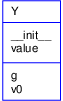
Figure 1 sketches the contents of class Y
as a so-called UML diagram, here created
with aid of the
program class_Y_v1_UML.py.
The UML diagram has two "boxes", one where the functions are listed,
and one where the variables are listed.
Our next step is to implement this class in Python.
Figure 1: UML diagram with function and data in the simple class Y for representing a mathematical function \( y(t;v_0) \).
Implementation
The complete code for our
class Y looks as follows in Python:
class Y:
    def __init__(self, v0):
        self.v0 = v0
        self.g = 9.81

    def value(self, t):
        return self.v0*t - 0.5*self.g*t**2
A puzzlement for newcomers to Python classes is the self
parameter, which may take some efforts and time to fully understand.
Usage and dissection
Before we dig into what each line in the class implementation means, we start by showing how the class can be used to compute values of the mathematical function \( y(t;v_0) \).
A class creates a new data type, here of name Y,
so when we use the class to make
objects, those objects are of type Y. (Actually,
all the standard Python objects, such as
lists, tuples, strings, floating-point numbers, integers,
etc., are built-in
Python classes, with names list, tuple,
str, float,
int, etc.)
An object of a user-defined class (like Y) is usually called
an instance.
We need such an instance in order to use the data in the class and call the
value function.
The following statement constructs an instance bound to the variable
name y:
y = Y(3)
Seemingly, we call the class Y as if it were a function.
Actually, Y(3) is automatically translated by Python to
a call to the constructor __init__ in class Y.
The arguments in the call, here only the number 3,
are always passed on as
arguments to __init__ after the self
argument. That is, v0 gets the value 3 and self
is just dropped in the call. This may be confusing, but it is a rule
that the self argument is never used in calls to
functions in classes.
With the instance y, we can compute the value \( y(t=0.1;v_0=3) \) by the
statement
v = y.value(0.1)
Here also, the self argument is dropped in the call to value.
To access functions and variables in a class, we must prefix the
function and variable names by the name of the instance and a dot:
the value function is reached as y.value, and the
variables are reached as y.v0 and y.g. We can, for example,
print the value of v0 in the instance y by writing
print y.v0
The output will in this case be 3.
We have already introduced the term "instance'' for the object of a class.
Functions in classes are commonly called methods,
and variables (data) in classes are called
data attributes. Methods are also known as method attributes.
From now on we will use this terminology. In our sample class Y
we have two methods or method attributes, __init__ and value, two
data attributes, v0 and g, and
four attributes
in total (__init__, value, v0, and g).
The names of attributes can be chosen freely, just as
names of ordinary Python functions and variables. However, the constructor
must have the name __init__, otherwise it is not automatically
called when we create new instances.
You can do whatever you want in whatever method, but it is a common convention to use the constructor for initializing the variables in the class.
Extension of the class
We can have as many attributes as we like in a class, so
let us add a new method to class Y. This method is called
formula and prints a string containing the formula of
the mathematical function \( y \). After this formula, we provide the
value of \( v_0 \). The string can then be
constructed as
'v0*t - 0.5*g*t**2; v0=%g' % self.v0
where self is an instance of class Y.
A call of formula does not need any arguments:
print y.formula()
should be enough to create, return, and print the string.
However, even if the formula method does not need any arguments, it
must have a self argument, which is left out in the call
but needed inside the method to access the attributes.
The implementation of the method is therefore
    def formula(self):
        return 'v0*t - 0.5*g*t**2; v0=%g' % self.v0
For completeness, the whole class now reads
class Y:
    def __init__(self, v0):
        self.v0 = v0
        self.g = 9.81

    def value(self, t):
        return self.v0*t - 0.5*self.g*t**2

    def formula(self):
        return 'v0*t - 0.5*g*t**2; v0=%g' % self.v0
Example on use may be
y = Y(5)
t = 0.2
v = y.value(t)
print 'y(t=%g; v0=%g) = %g' % (t, y.v0, v)
print y.formula()
with the output
y(t=0.2; v0=5) = 0.8038
v0*t - 0.5*g*t**2; v0=5
class headline.
Ordinary data attribute assignment must be done inside methods.
The main program using the class must appear with the same indent as
the class headline.
Using methods as ordinary functions
We may create several \( y \) functions with different values of \( v_0 \):
y1 = Y(1)
y2 = Y(1.5)
y3 = Y(-3)
We can treat y1.value, y2.value, and
y3.value as ordinary Python functions of t, and then pass
them on to any Python function that expects a function of one variable.
In particular, we can send the functions to the diff(f, x) function
from the section Challenge: functions with parameters:
dy1dt = diff(y1.value, 0.1)
dy2dt = diff(y2.value, 0.1)
dy3dt = diff(y3.value, 0.2)
Inside the diff(f, x) function, the argument
f now behaves as a function
of one variable that automatically
carries with it two variables v0 and g.
When f refers to (e.g.) y3.value, Python actually
knows that f(x)
means y3.value(x), and inside the y3.value method
self is y3, and we have
access to y3.v0 and y3.g.
New-style classes versus classic classes
When use Python version 2 and write a class like
class V:
    ...
we get what is known as an old-style or classic class. A revised
implementation of classes in Python came in version 2.2 with
new-style classes. The specification of a new-style class requires
(object) after the class name:
class V(object):
    ...
New-style classes have more functionality, and it is in general recommended
to work with new-style classes.
We shall therefore from now write V(object) rather than just V.
In Python 3, all classes are new-style whether we write V or V(object).
Doc strings
A function may have a doc string right after the
function definition, see the section ref{sec:basic:docstring}.
The aim of the doc string is to explain the purpose of the function
and, for instance, what the arguments and return values are.
A class can also have a doc string, it is just the first string that
appears right after the class headline.
The convention is to enclose the doc string in triple double quotes """:
class Y(object):
    """The vertical motion of a ball."""

    def __init__(self, v0):
        ...
More comprehensive information can include the methods and how the class is used in an interactive session:
class Y(object):
    """
    Mathematical function for the vertical motion of a ball.

    Methods:
       constructor(v0): set initial velocity v0.
       value(t): compute the height as function of t.
       formula(): print out the formula for the height.

    Data attributes:
       v0: the initial velocity of the ball (time 0).
       g: acceleration of gravity (fixed).

    Usage:
    >>> y = Y(3)
    >>> position1 = y.value(0.1)
    >>> position2 = y.value(0.3)
    >>> print y.formula()
    v0*t - 0.5*g*t**2; v0=3
    """
The self variable
Now we will provide some more explanation of the self parameter and
how the class methods work. Inside the constructor __init__, the
argument self is a variable holding the new instance to be
constructed. When we write
    self.v0 = v0
    self.g = 9.81
we define two new data attributes in this instance. The self parameter
is invisibly returned to the calling code. We can imagine that Python
translates the syntax y = Y(3) to a call written as
Y.__init__(y, 3)
Now, self becomes the new instance y we want to create, so when we
do self.v0 = v0 in the constructor, we actually assign v0 to
y.v0. The prefix with Y. illustrates how to reach a class method
with a syntax similar to reaching a function in a module (just like
math.exp). If we prefix with Y., we need to explicitly feed in an
instance for the self argument, like y in the code line above, but
if we prefix with y. (the instance name) the self argument is
dropped in the syntax, and Python will automatically assign the y
instance to the self argument. It is the latter "instance name
prefix" which we shall use when computing with
classes. (Y.__init__(y, 3) will not work since y is undefined and
supposed to be an Y object. However, if we first create y = Y(2)
and then call Y.__init__(y, 3), the syntax works, and y.v0 is 3
after the call.)
Let us look at a call to the value method to see a similar
use of the self argument. When we write
value = y.value(0.1)
Python translates this to a call
value = Y.value(y, 0.1)
such that the self argument in the value method becomes
the y instance. In the expression inside the value method,
self.v0*t - 0.5*self.g*t**2
self is y so this is the same as
y.v0*t - 0.5*y.g*t**2
The use of self may become more apparent when we have multiple class
instances. We can make a class that just has one parameter so we
can easily identify a class instance by printing the value of this
parameter. In addition, every Python object obj has a unique
identifier obtained by id(obj) that we can also print to track
what self is.
class SelfExplorer(object):
    def __init__(self, a):
        self.a = a
        print 'init: a=%g, id(self)=%d' % (self.a, id(self))

    def value(self, x):
        print 'value: a=%g, id(self)=%d' % (self.a, id(self))
        return self.a*x
Here is an interactive session with this class:
>>> s1 = SelfExplorer(1)
init: a=1, id(self)=38085696
>>> id(s1)
38085696
We clearly see that self inside the constructor is the same
object as s1, which we want to create by calling the constructor.
A second object is made by
>>> s2 = SelfExplorer(2)
init: a=2, id(self)=38085192
>>> id(s2)
38085192
Now we can call the value method using the standard syntax s1.value(x)
and the "more pedagogical" syntax SelfExplorer.value(s1, x).
Using both s1 and s2 illustrates how self take on different
values, while we may look at the method SelfExplorer.value as
a single function that just operates on different self and x
objects:
>>> s1.value(4)
value: a=1, id(self)=38085696
4
>>> SelfExplorer.value(s1, 4)
value: a=1, id(self)=38085696
4

>>> s2.value(5)
value: a=2, id(self)=38085192
10
>>> SelfExplorer.value(s2, 5)
value: a=2, id(self)=38085192
10
Hopefully, these illustrations help to explain that self is just
the instance used in the method call prefix, here s1 or s2.
If not, patient work with class programming in Python will over
time reveal an understanding of what self really is.
self.
- Any class method must have
selfas first argument. (The name can be any valid variable name, but the nameselfis a widely established convention in Python.) -
selfrepresents an (arbitrary) instance of the class. - To access any class attribute inside class methods, we must prefix with
self, as inself.name, wherenameis the name of the attribute. -
selfis dropped as argument in calls to class methods.
Another function class example
Let us apply the ideas from the Y class to the function
$$
\begin{equation*}
v(r) = \left({\beta\over 2\mu_0}\right)^{{1/ n}}
{n \over n+1}\left( R^{1 + 1/n} - r^{1 + 1/n}\right) ,
\end{equation*}
$$
where \( r \) is the independent variable.
We may write this function as \( v(r; \beta,\mu_0,n,R) \) to
explicitly indicate that
there is one primary independent variable (\( r \)) and four physical
parameters \( \beta \), \( \mu_0 \), \( n \), and \( R \).
The class typically holds
the physical parameters as variables and provides an value(r) method
for computing the \( v \) function:
class V(object):
    def __init__(self, beta, mu0, n, R):
        self.beta, self.mu0, self.n, self.R = beta, mu0, n, R

    def value(self, r):
        beta, mu0, n, R = self.beta, self.mu0, self.n, self.R
        n = float(n)  # ensure float divisions
        v = (beta/(2.0*mu0))**(1/n)*(n/(n+1))*\
            (R**(1+1/n) - r**(1+1/n))
        return v
There is seemingly one new thing here in that we initialize several variables on the same line:
self.beta, self.mu0, self.n, self.R = beta, mu0, n, R
The comma-separated list of variables on the right-hand side forms a tuple so this assignment is just the a valid construction where a set of variables on the left-hand side is set equal to a list or tuple on the right-hand side, element by element. An equivalent multi-line code is
        self.beta = beta
        self.mu0 = mu0
        self.n = n
        self.R = R
In the value method it is convenient to avoid the
self. prefix in the mathematical formulas and instead introduce
the local short names beta, mu0, n, and R.
This is in general a good idea, because it makes it easier to read the
implementation of the formula and check its correctness.
Remark
Another solution to the problem of sending functions with parameters
to a general library function such as diff is provided in
the document Variable number of
function arguments in Python
[2]. The remedy there is to transfer the
parameters as arguments "through" the diff function. This can be
done in a general way as explained in that appendix.
Alternative function class implementations
To illustrate class programming further, we will now realize class
Y from the section Representing a function as a class in a different way.
You may consider this section as advanced and skip it, but for
some readers the material might improve the understanding of
class Y and give some insight into
class programming in general.
It is a good habit always to have a constructor in a class and to
initialize the data attributes in the class here, but this is not a
requirement. Let us drop the constructor and make v0 an optional
argument to the value method. If the user does not provide v0 in
the call to value, we use a v0 value that must have been provided
in an earlier call and stored as a data attribute self.v0. We can
recognize if the user provides v0 as argument or not by using None
as default value for the keyword argument and then test if v0 is
None.
Our alternative implementation of class Y, named Y2, now reads
class Y2(object):
    def value(self, t, v0=None):
        if v0 is not None:
            self.v0 = v0
        g = 9.81
        return self.v0*t - 0.5*g*t**2
This time the class has only one method and one data attribute as we
skipped the constructor and let g be a local variable in
the value method.
But if there is no constructor, how is an instance created? Python fortunately creates an empty constructor. This allows us to write
y = Y2()
to make an instance y. Since nothing happens in the automatically
generated empty constructor, y has no data attributes at this stage.
Writing
print y.v0
therefore leads to the exception
AttributeError: Y2 instance has no attribute 'v0'
By calling
v = y.value(0.1, 5)
we create an attribute self.v0 inside the value method.
In general, we can create any attribute name in any method by just assigning
a value to self.name. Now trying a
print y.v0
will print 5.
In a new call,
v = y.value(0.2)
the previous v0 value (5) is used inside value as
self.v0 unless a v0 argument is specified in the call.
The previous implementation is not foolproof if we fail to initialize
v0. For example, the code
y = Y2()
v = y.value(0.1)
will terminate in the value method with the exception
AttributeError: Y2 instance has no attribute 'v0'
As usual, it is better to notify the user with a more informative message.
To check if we have an attribute v0, we can use the Python
function hasattr. Calling hasattr(self, 'v0') returns
True only if the instance self has an attribute
with name 'v0'. An improved value method now reads
    def value(self, t, v0=None):
        if v0 is not None:
            self.v0 = v0
        if not hasattr(self, 'v0'):
            print 'You cannot call value(t) without first '\
                  'calling value(t,v0) to set v0'
            return None
        g = 9.81
        return self.v0*t - 0.5*g*t**2
Alternatively, we can try to
access self.v0 in a try-except block, and
perhaps raise an exception TypeError (which is what Python raises if
there are not enough arguments to a function or method):
    def value(self, t, v0=None):
        if v0 is not None:
            self.v0 = v0
        g = 9.81
        try:
            value = self.v0*t - 0.5*g*t**2
        except AttributeError:
            msg = 'You cannot call value(t) without first '
                  'calling value(t,v0) to set v0'
            raise TypeError(msg)
        return value
Note that Python detects an AttributeError, but from a user's
point of view, not enough parameters were supplied in the call so
a TypeError is more appropriate to communicate back to the
calling code.
We think class Y is a better implementation than class Y2,
because the former is simpler. As already mentioned, it
is a good habit to include
a constructor and set data here rather than "recording data on the fly"
as we try to in class Y2. The whole purpose of class Y2
is just to show that Python provides great flexibility with respect
to defining attributes, and that there are no requirements to what
a class must contain.
Making classes without the class construct
Newcomers to the class concept often have a hard time understanding what this concept is about. The present section tries to explain in more detail how we can introduce classes without having the class construct in the computer language. This information may or may not increase your understanding of classes. If not, programming with classes will definitely increase your understanding with time, so there is no reason to worry. In fact, you may safely jump to the section Special methods as there are no important concepts in this section that later sections build upon.
A class contains a collection of variables (data) and a collection of methods (functions). The collection of variables is unique to each instance of the class. That is, if we make ten instances, each of them has its own set of variables. These variables can be thought of as a dictionary with keys equal to the variable names. Each instance then has its own dictionary, and we may roughly view the instance as this dictionary. (The instance can also contain static data attributes (the section Static methods and attributes), but these are to be viewed as global variables in the present context.)
On the other hand, the methods are shared
among the instances. We may think of a method in a class
as a standard global
function that takes an instance in the form of a dictionary
as first
argument. The method has then access to the variables in the instance
(dictionary) provided in the call.
For the Y class from the section Representing a function as a class
and an instance y,
the methods are ordinary
functions with the following names and arguments:
Y.value(y, t)
Y.formula(y)
The class acts as a namespace,
meaning that all functions
must be prefixed by the namespace name, here Y.
Two different classes, say C1 and C2, may have functions
with the same name, say value, but when the value functions
belong to different namespaces, their names C1.value and
C2.value become distinct.
Modules are also namespaces for the functions and variables in them
(think of math.sin, cmath.sin, numpy.sin).
The only peculiar thing with the class construct in Python is that it allows us to use an alternative syntax for method calls:
y.value(t)
y.formula()
This syntax coincides with the traditional syntax of calling class
methods and providing arguments, as found in other computer languages,
such as Java, C#, C++, Simula, and Smalltalk.
The dot notation is also used to access variables in an instance
such that we inside a method can write self.v0 instead of
self['v0'] (self refers to y through the function call).
We could easily
implement a simple version of the class concept without having a class
construction in the language. All we need is a dictionary type and
ordinary functions. The dictionary acts as the instance, and methods are
functions that take this dictionary as the first argument such that
the function has access to
all the variables in the instance.
Our Y class could now be implemented as
def value(self, t):
    return self['v0']*t - 0.5*self['g']*t**2

def formula(self):
    print 'v0*t - 0.5*g*t**2; v0=%g' % self['v0']
The two functions are placed in a module called Y.
The usage goes as follows:
import Y
y = {'v0': 4, 'g': 9.81}   # make an "instance"
y1 = Y.value(y, t)
We have no constructor since the initialization of the variables is
done when declaring the dictionary y, but we could well include
some initialization function in the Y module
def init(v0):
    return {'v0': v0, 'g': 9.81}
The usage is now slightly different:
import Y
y = Y.init(4)       # make an "instance"
y1 = Y.value(y, t)
This way of implementing classes with the aid of a dictionary and
a set of ordinary functions actually forms the basis for class implementations
in many languages. Python and Perl even
have a syntax that demonstrates this type of
implementation. In fact, every class instance in Python has a dictionary
__dict__ as attribute, which holds all the
variables in the instance. Here is a demo that proves the existence of this
dictionary in class Y:
>>> y = Y(1.2)
>>> print y.__dict__
{'v0': 1.2, 'g': 9.8100000000000005}
To summarize: A Python class can be thought of as some variables collected in a dictionary, and a set of functions where this dictionary is automatically provided as first argument such that functions always have full access to the class variables.
First remark
We have in this section provided a view of classes from a technical point of view. Others may view a class as a way of modeling the world in terms of data and operations on data. However, in sciences that employ the language of mathematics, the modeling of the world is usually done by mathematics, and the mathematical structures provide understanding of the problem and structure of programs. When appropriate, mathematical structures can conveniently be mapped on to classes in programs to make the software simpler and more flexible.
Second remark
The view of classes in this section neglects very important topics such as inheritance and dynamic binding (explained in the document Object-oriented programming [1]). For more completeness of the present section, we therefore briefly describe how our combination of dictionaries and global functions can deal with inheritance and dynamic binding (but this will not make sense unless you know what inheritance is).
Data inheritance can be obtained by letting a subclass dictionary
do an update call with the superclass dictionary as argument.
In this way all data in the superclass are also available in the
subclass dictionary. Dynamic binding of methods is more complicated, but
one can think of checking if the method is in the subclass module
(using hasattr), and if not, one proceeds with checking super
class modules until a version of the method is found.
Closures
This section follows up the discussion in the section Making classes without the class construct and presents a more advanced construction that may serve as alternative to class constructions in some cases.
Our motivating example is that we want a Python implementation of a mathematical function \( y(t;v_0)=v_0t - \frac{1}{2}gt^2 \) to have \( t \) as the only argument, but also have access to the parameter \( v_0 \). Consider the following function, which returns a function:
>>> def generate_y():
...     v0 = 5
...     g = 9.81
...     def y(t):
...         return v0*t - 0.5*g*t**2
...     return y
...
>>> y = generate_y()
>>> y(1)
0.09499999999999975
The remarkable property of the y function is that it remembers the
value of v0 and g, although these variables are not local to
the parent function generate_y and not local in y. In particular,
we can specify v0 as argument to generate_y:
>>> def generate_y(v0):
...     g = 9.81
...     def y(t):
...         return v0*t - 0.5*g*t**2
...     return y
...
>>> y1 = generate_y(v0=1)
>>> y2 = generate_y(v0=5)
>>> y1(1)
-3.9050000000000002
>>> y2(1)
0.09499999999999975
Here, y1(t) has access to v0=1 while y2(t) has access to v0=5.
The function y(t) we construct and return from generate_y is
called a closure and it remembers the value of the surrounding
local variables in the parent function (at the time we create the
y function). Closures are very convenient for many
purposes in mathematical computing.
Examples appear in the section Example: Automagic differentiation.
Closures are also central in
a programming style called functional programming.
Let us generate a series of functions v(t) for various
values of a parameter v0. Each function just returns
a tuple (v0, t) such that we can easily see what the argument and
the parameter are. We use lambda to quickly define
each function, and we place the functions in a list:
>>> def generate():
...     return [lambda t: (v0, t) for v0 in [0, 1, 5, 10]]
...
>>> funcs = generate()
Now, funcs is a list of functions with one argument.
Calling each function and printing
the return values v0 and t gives
>>> for func in funcs:
...     print func(1)
...
(10, 1)
(10, 1)
(10, 1)
(10, 1)
As we see, all functions have v0=10, i.e., they stored the most recent
value of v0 before return. This is not what we wanted.
The trick is to let v0 be a keyword argument in each function,
because the value of a keyword argument is frozen at the time the
function is defined:
>>> def generate():
...     return [lambda t, v0=v0: (v0, t)
...             for v0 in [0, 1, 5, 10]]
...
>>> funcs = generate()
>>> for func in funcs:
...     print func(1)
...
(0, 1)
(1, 1)
(5, 1)
(10, 1)