`odespy`¶

The odespy package contains tools for solving ordinary differential equations (ODEs). The user specifies the problem through high-level Python code. Both scalar ODEs and systems of ODEs are supported. A wide range of numerical methods for ODEs are offered:

Classname	Short description
AdamsBashMoulton2	Explicit 2nd-order Adams-Bashforth-Moulton method
AdamsBashMoulton3	Explicit 3rd-order Adams-Bashforth-Moulton method
AdamsBashforth2	Explicit 2nd-order Adams-Bashforth method
AdamsBashforth3	Explicit 3rd-order Adams-Bashforth method
AdamsBashforth4	Explicit 4th-order Adams-Bashforth method
AdaptiveResidual	Very simple adaptive strategy based on the residual
Backward2Step	Implicit 2nd-order Backward Euler method
BackwardEuler	Implicit 1st-order Backward Euler method
BogackiShampine	Adaptive Bogacki-Shampine RK method of order (3, 2)
CashKarp	Adaptive Cash-Karp RK method of order (5, 4)
Dop853	Adaptive Dormand & Prince method of order 8(5,3) (scipy)
Dopri5	Dormand & Prince method of order 5(4) (scipy)
DormandPrince	Dormand & Prince RK method of order (5, 4)
Euler	The simple explicit (forward) Euler scheme
Fehlberg	Adaptive Runge-Kutta-Fehlberg (4,5) method
ForwardEuler	The simple explicit (forward) Euler scheme
Heun	Heun’s explicit method (similar to RK2)
Leapfrog	Standard explicit Leapfrog scheme
LeapfrogFiltered	Filtered Leapfrog scheme
Lsoda	LSODA solver with stiff-nonstiff auto shift
Lsodar	LSODAR method with stiff-nonstiff auto shift
Lsode	LSODE solver for a stiff or nonstiff system
Lsodes	LSODES solver for sparse Jacobians
Lsodi	LSODI solver for linearly implicit systems
Lsodis	LSODIS solver for linearly implicit sparse systems
Lsoibt	LSOIBIT solver for linearly implicit block tridiag systems
MidpointImplicit	Implicit 2nd-order Midpoint method
MidpointIter	Explicit 2nd-order iterated Midpoint method
RK2	Explicit 2nd-order Runge-Kutta method
RK3	Explicit 3rd-order Runge-Kutta method
RK34	Adaptive 4th-order Runge-Kutta method
RK4	Explicit 4th-order Runge-Kutta method
RKC	Explicit 2nd-order Runge-Kutta-Chebyshev method (rkc.f)
RKF45	Adaptive Runge-Kutta-Fehlberg (4,5) method (rkf45.f)
RKFehlberg	Adaptive Runge-Kutta-Fehlberg (4,5) method
RungeKutta1	Explicit 1st-order Runge-Kutta method
RungeKutta2	Explicit 2nd-order Runge-Kutta method
RungeKutta3	Explicit 3rd-order Runge-Kutta method
RungeKutta4	Explicit 4th-order Runge-Kutta method
ThetaRule	Unified Forward/Backward Euler and Midpoint methods
Trapezoidal	Heun’s explicit method (similar to RK2)
Vode	Adams/BDF Vode adaptive method (vode.f wrapper)
lsoda_scipy	Wrapper of lsoda (scipy.integrate.odeint)
odefun_sympy	Very accurate high order Taylor method (from SymPy)
odelab	interface to all solvers in odelab

Basic Usage¶

This section explains how to use Odespy. The general principles and program steps are first explained and then followed by a series of examples with progressive complexity with respect to Python constructs and numerical methods.

Overview¶

A code using Odespy to solve ODEs consists of six steps. These are outlined in generic form below.

Step 1¶

Write the ODE problem in generic form $u' = f(u, t)$, where $u(t)$ is the unknown function to be solved for, or a vector of unknown functions of time in case of a system of ODEs.

Step 2¶

Implement the right-hand side function $f(u, t)$ as a Python function f(u, t). The argument u is either a float object, in case of a scalar ODE, or a numpy array object, in case of a system of ODEs. Some solvers in this package also allow implementation of $f$ in FORTRAN for increased efficiency.

Step 3¶

Create a solver object

solver = classname(f)

where classname is the name of a class in this package implementing the desired numerical method.

Many solver classes has a range of parameters that the user can set to control various parts of the solution process. The parameters are documented in the doc string of the class (pydoc classname will list the documentation in a terminal window). One can either specify parameters at construction time, via extra keyword arguments to the constructor,

solver = classname(f, prm1=value1, prm2=value2, ...)

or at any time using the set method:

solver.set(prm1=value1, prm2=value2, prm3=value3)
...
solver.set(prm4=value4)

Step 4¶

Set the initial condition $u(0)=U_0$,

solver.set_initial_condition(U0)

where U0 is either a number, for a scalar ODE, or a sequence (list, tuple, numpy array), for a system of ODEs.

Step 5¶

Solve the ODE problem, which means to compute $u(t)$ at some discrete user-specified time points $t_1, t_2, \ldots, t_N$.

T = ...  # end time
time_points = numpy.linspace(0, T, N+1)
u, t = solver.solve(time_points)

In case of a scalar ODE, the returned solution u is a one-dimensional numpy array where u[i] holds the solution at time point t[i]. For a system of ODEs, the returned u is a two-dimensional numpy array where u[i,j] holds the solution of the $j$-th unknown function at the $i$-th time point t[i] ($u_j(t_i)$ in mathematics notation).

By giving the parameter disk_storage=True to the solver’s constructor, the returned u array is memory mapped (i.e., of type numpy.memmap) such that all the data are stored on file, but parts of the array can be efficiently accessed.

The time_points array specifies the time points where we want the solution to be computed. The returned array t is the same as time_points. The simplest numerical methods in the Odespy package apply the time_points array directly for the time stepping. That is, the time steps used are given by

time_points[i] - time_points[i-1]  #  i=0,1,...,len(time_points)-1

The adaptive schemes typically compute between each time point in the time_points array, making this array a specification where values of the unknowns are desired.

The solve method in solver classes also allows a second argument, terminate, which is a user-implemented Python function specifying when the solution process is to be terminated. For example, terminating when the solution reaches an asymptotic (known) value a can be done by

def terminate(u, t, step_no):
    # u and t are arrays. Most recent solution is u[step_no].
    tolerance = 1E-6
    return abs(u[step_no] - a) < tolerance

u, t = solver.solve(time_points, terminate)

The arguments transferred to the terminate function are the solution array u, the corresponding time points t, and an integer step_no reflecting the most recently computed u value. That is, u[step_no] is most recently computed value of $u$. (The array data u[step_no+1:] will typically be zero as these are uncomputed future values.)

Step 6¶

Extract solution components for plotting and further analysis. Since the u array returned from solver.solve stores all unknown functions at all discrete time levels, one usually wants to extract individual unknowns as one-dimensional arrays. Here is an example where unknown number $0$ and $k$ are extracted in individual arrays and plotted:

u_0 = u[:,0]
u_k = u[:,k]

from matplotlib.pyplot import plot, show
plot(t, u_0, t, u_k)
show()

First Example: Logistic Growth¶

Our first example concerns the simple scalar ODE problem

\[\frac{du}{dt}=au\left(1-\frac{u}{R}\right),\quad u(0)=A,\]

where $A>0$, $a>0$, and $R>0$ are known constants. This is a common model for population dynamics in ecology where $u$ is the number of individuals, $a$ the initial growth rate, $R$ is the maximum number of individuals that the environment allows (the so-called carrying capacity of the environment).

Using a standard Runge-Kutta method of order four, the code for solving the problem in the time interval $[0,10]$ with $N=30$ time steps, looks like this (program logistic1.py):

def f(u, t):
    return a*u*(1 - u/R)

a = 2
R = 1E+5
A = 1

import odespy
solver = odespy.RK4(f)
solver.set_initial_condition(A)

from numpy import linspace, exp
T = 10  # end of simulation
N = 30  # no of time steps
time_points = linspace(0, T, N+1)
u, t = solver.solve(time_points)

With the RK4 method and other non-adaptive methods the time steps are dictated by the time_points array. A constant time step of size is implied in the present example. Running an alternative numerical method just means replacing RK4 by, e.g., RK2, ForwardEuler, BackwardEuler, AdamsBashforth2, etc.

We can easily plot the numerical solution and compare with the exact solution (which is known for this equation):

def u_exact(t):
    return R*A*exp(a*t)/(R + A*(exp(a*t) - 1))

from matplotlib.pyplot import *

plot(t, u, 'r-',
     t, u_exact(t), 'bo')
savefig('tmp.png')
show()

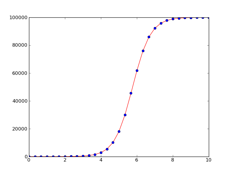
Solution of the logistic equation with the 4-th order Runge-Kutta method (solid line) and comparison with the exact solution (dots)

All the examples in this tutorial are found in the GitHub directory https://github.com/hplgit/odespy/tree/master/doc/src/odespy/src-odespy/. If you download the tarball or clone the GitHub repository, the examples reside in the directory doc/src/odespy/src-odespy.

Parameters in the Right-Hand Side Function¶

The right-hand side function and all physical parameters are often lumped together in a class, for instance,

class Logistic:
    def __init__(self, a, R, A):
        self.a = a
        self.R = R
        self.A = A

    def f(self, u, t):
        a, R = self.a, self.R  # short form
        return a*u*(1 - u/R)

    def u_exact(self, t):
        a, R, A = self.a, self.R, self.A  # short form
        return R*A*exp(a*t)/(R + A*(exp(a*t) - 1))

Note that introducing local variables like a and R, instead of using self.a and self.A, makes the code closer to the mathematics. This can be convenient when proof reading the implementation of complicated ODEs.

The numerical solution is computed by

import odespy
problem = Logistic(a=2, R=1E+5, A=1)
solver = odespy.RK4(problem.f)
solver.set_initial_condition(problem.A)

T = 10  # end of simulation
N = 30  # no of time steps
time_points = linspace(0, T, N+1)
u, t = solver.solve(time_points)

The complete program is available in the file program logistic2.py.

Instead of having the problem parameters a and R in the ODE as global variables or in a class, we may include them as extra arguments to f, either as positional arguments or as keyword arguments. Positional arguments can be sent to f via the constructor argument f_args (a list/tuple of variables), while a dictionary f_kwargs is used to transfer keyword arguments to f via the constructor. Here is an example on using keyword arguments:

def f(u, t, a=1, R=1):
    return a*u*(1 - u/R)

A = 1

import odespy
solver = odespy.RK4(f, f_kwargs=dict(a=2, R=1E+5))

In general, a mix of positional and keyword arguments can be used in f:

def f(u, t, arg1, arg2, arg3, ..., kwarg1=val1, kwarg2=val2, ...):
    ...

solver = odespy.classname(f,
                    f_args=[arg1, arg2, arg3, ...],
                    f_kwargs=dict(kwarg1=val1, kwarg2=val2, ...))

# Alternative setting of f_args and f_kwargs
solver.set(f_args=[arg1, arg2, arg3, ...],
           f_kwargs=dict(kwarg1=val1, kwarg2=val2, ...))

Solvers will call f as f(u, t, *f_args, **f_kwargs).

Termination Criterion for the Simulation¶

We know that the solution $u$ of the logistic equation approaches $R$ as $t\rightarrow\infty$. Instead of using a trial and error process for determining an appropriate time integral for integration, the solver.solve method accepts a user-defined function terminate that can be used to implement a criterion for terminating the solution process. Mathematically, the relevant criterion is $||u-R||<\hbox{tol}$, where tol is an acceptable tolerance, say $100$ in the present case where $R=10^5$. The terminate function implements the criterion and returns true if the criterion is met:

def terminate(u, t, step_no):
    """u[step_no] holds (the most recent) solution at t[step_no]."""
    return abs(u[step_no] - R) < tol:

Note that the simulation is anyway stopped for $t > T$ so $T$ must be large enough for the termination criterion to be reached (if not, a warning will be issued). With a terminate function it is also convenient to specify the time step dt and not the total number of time steps.

A complete program can be as follows (logistic5.py):

def f(u, t):
    return a*u*(1 - u/R)

a = 2
R = 1E+5
A = 1

import odespy, numpy
solver = odespy.RK4(f)
solver.set_initial_condition(A)

T = 20  # end of simulation
dt = 0.25
N = int(round(T/dt))
time_points = numpy.linspace(0, T, N+1)

tol = 100   # tolerance for termination criterion

def terminate(u, t, step_no):
    """u[step_no] holds (the most recent) solution at t[step_no]."""
    return abs(u[step_no] - R) < tol:

u, t = solver.solve(time_points, terminate)
print 'Final u(t=%g)=%g' % (t[-1], u[-1])

from matplotlib.pyplot import *
plot(t, u, 'r-')
savefig('tmp.png')
show()

A Class-Based Implementation¶

The previous code example can be recast into a more class-based (“object-oriented programming”) example. We lump all data related to the problem (the “physics”) into a problem class Logistic, while all data related to the numerical solution and its quality are taken care of by class Solver. The code below illustrates the ideas (logistic6.py):

import numpy as np
import matplotlib.pyplot as mpl
import odespy

class Logistic:
    def __init__(self, a, R, A, T):
        """
        `a` is (initial growth rate), `R` the carrying capacity,
        `A` the initial amount of u, and `T` is some (very) total
        simulation time when `u` is very close to the asymptotic
        value `R`.
        """
        self.a, self.R, self.A = a, R, A
        self.tol = 0.01*R # tolerance for termination criterion

    def f(self, u, t):
        """Right-hand side of the ODE."""
        a, R = self.a, self.R  # short form
        return a*u*(1 - u/R)

    def terminate(self, u, t, step_no):
        """u[step_no] holds solution at t[step_no]."""
        return abs(u[step_no] - self.R) < self.tol

    def u_exact(self, t):
        a, R, A = self.a, self.R, self.A  # short form
        return R*A*np.exp(a*t)/(R + A*(np.exp(a*t) - 1))


class Solver:
    def __init__(self, problem, dt, method='RK4'):
        self.problem = problem
        self.dt = dt
        self.method_class = eval('odespy.' + method)
        self.N = int(round(T/dt))

    def solve(self):
        self.solver = self.method_class(self.problem.f)
        self.solver.set_initial_condition(self.problem.A)
        time_points = np.linspace(0, self.problem.T, self.N+1)
        self.u, self.t = self.solver.solve(
            time_points, self.problem.terminate)
        print 'Final u(t=%g)=%g' % (t[-1], u[-1])

    def plot(self):
        mpl.plot(self.t, self.u, 'r-',
                 self.t, self.u_exact(self.t), 'bo')
        mpl.legend(['numerical', 'exact'])
        mpl.savefig('tmp.png')
        mpl.show()

def main():
    problem = Logistic(a=2, R=1E+5, A=1, T=20)
    solver = Solver(problem, dt=0.25, method='RK4')
    solver.solve()
    solver.plot()

if __name__ == '__main__':
    main()

Using Other Symbols¶

The Odespy package applies u for the unknown function or vector of unknown functions and t as the name of the independent variable. Many problems involve other symbols for functions and independent variables. These symbols should be reflected in the user’s code. For example, here is a coding example involving the logistic equation written as $y'(x)=au(x)(1-u(x)/R(x))$, where now a variable $R=R(x)$ is considered. Following the setup from the very first program above solving the logistic ODE, we can easily introduce our own nomenclature (logistic7.py):

def f(y, x):
    return a*y*(1 - y/R)

a = 2;  R = 1E+5;  A = 1

import odespy, numpy
solver = odespy.RK4(f)
solver.set_initial_condition(A)

L = 10  # end of x domain
N = 30  # no of time steps
x_points = numpy.linspace(0, L, N+1)
y, x = solver.solve(x_points)

from matplotlib.pyplot import *
plot(x, y, 'r-')
xlabel('x'); ylabel('y')
show()

As shown, we use y for u, x for t, and x_points instead of time_points.

Example: Solving an ODE System¶

We shall now explain how to solve a system of ODEs using a scalar second-order ODE as starting point. The angle $\theta$ of a pendulum with mass $m$ and length $L$ is governed by the equation (neglecting air resistance for simplicity)

\[mL\ddot\theta + mg\sin\theta = 0,\quad \theta (0)=\Theta,\ \dot\theta (0)=0 .\]

A dot over $\theta$ implies differentiation with respect to time. The ODE can be written as $\ddot\theta + c\sin\theta=0$ by introducing $c = g/L$. This problem must be expressed as a first-order ODE system if it is going to be solved by the tools in the Odespy package. Introducing $\omega = \dot\theta$ (the angular velocity) as auxiliary unknown, we get the system

\[\begin{split}\dot\theta &= \omega,\\ \dot\omega &= -c\sin\theta,\end{split}\]

with $\theta(0)=\Theta$ and $\omega(0)=0$.

Now the f function must return a list or array with the two right-hand side functions:

def f(u, t):
    theta, omega = u
    return [omega, -c*sin(theta)]

Note that when we have a system of ODEs with n components, the u object sent to the f function is an array of length n, representing the value of all components in the ODE system at time t. Here we extract the two components of u in separate local variables with names equal to what is used in the mathematical description of the current problem.

The initial conditions must be specified as a list:

solver = odespy.Heun(f)
solver.set_initial_condition([Theta, 0])

To specify the time points we here first decide on a number of periods (oscillations back and forth) to simulate and then on the time resolution of each period. Note that when $\Theta$ is small we can replace $\sin\theta$ by $\theta$ and find an analytical solution $\theta (t)=\Theta\cos\left(\sqrt{c}t\right)$ whose period is $2\pi/\sqrt{c}$. We use this expression as an approximation for the period also when $\Theta$ is not small.

freq = sqrt(c)      # frequency of oscillations when Theta is small
period = 2*pi/freq  # the period of the oscillations
T = 10*period       # final time
N_per_period = 20   # resolution of one period
N = N_per_period*period
time_points = numpy.linspace(0, T, N+1)

u, t = solver.solve(time_points)

The u returned from solver.solve is a two-dimensional array, where the columns hold the various solution functions of the ODE system. That is, the first column holds $\theta$ and the second column holds $\omega$. For convenience we extract the individual solution components in individual arrays:

theta = u[:,0]
omega = u[:,1]

from matplotlib.pyplot import *
plot(t, theta, 'r-')
savefig('tmp.png')
show()

The complete program is available in the file osc1a.py.

Looking at the plot reveals that the numerical solution has an alarming feature: the amplitude grows (indicating increasing energy in the system). Changing T to 28 periods instead of 10 makes the numerical solution explode. The increasing amplitude is a numerical artifact that some of the simple solution methods suffer from.

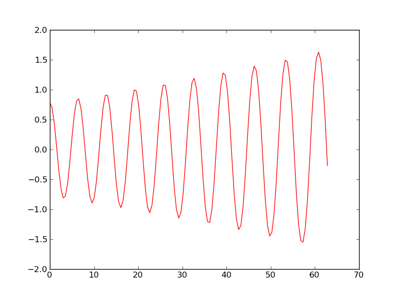
Heun’s method used to simulate oscillations of a pendulum

Using a more sophisticated method, say the 4-th order Runge-Kutta method, is just a matter of substituting Heun by RK4:

solver = odespy.RK4(f)
solver.set_initial_condition([Theta, 0])
freq = sqrt(c)      # frequency of oscillations when Theta is small
period = 2*pi/freq  # the period of the oscillations
T = 10*period       # final time
N_per_period = 20   # resolution of one period
N = N_per_period*period
time_points = numpy.linspace(0, T, N+1)

u, t = solver.solve(time_points)

theta = u[:,0]
omega = u[:,1]

from matplotlib.pyplot import *
plot(t, theta, 'r-')
savefig('tmp.png')
show()

The amplitude now becomes constant in time as expected.

Testing Several Methods¶

We shall now make a more advanced solver by extending the previous example. More specifically, we shall

represent the right-hand side function as class,

compare several different solvers,

compute error of numerical solutions.

Since we want to compare numerical errors in the various solvers we need a test problem where the exact solution is known. Approximating $\sin(\theta)$ by $\theta$ (valid for small $\theta$), gives the ODE system

\[\begin{split}\dot\theta &= \omega,\\ \dot\omega &= -c\theta,\end{split}\]

with $\theta(0)=\Theta$ and $\omega(0)=0$.

Right-hand side functions with parameters can be handled by including extra arguments via the f_args and f_kwargs functionality, or by using a class where the parameters are attributes and an f method defines $f(u,t)$. The section Parameters in the Right-Hand Side Function exemplifies the details. A minimal class representation of the right-hand side function in the present case looks like this:

class Problem:
    def __init__(self, c, Theta):
        self.c, self.Theta = float(c), float(Theta)

    def f(self, u, t):
        theta, omega = u;  c = self.c
        return [omega, -c*theta]

problem = Problem(c=1, Theta=pi/4)

It would be convenient to add an attribute period which holds an estimate of the period of oscillations as we need this for deciding on the complete time interval for solving the differential equations. An appropriate extension of class Problem is therefore

class Problem:
    def __init__(self, c, Theta):
        self.c, self.Theta = float(c), float(Theta)

        self.freq = sqrt(c)
        self.period = 2*pi/self.freq

    def f(self, u, t):
        theta, omega = u;  c = self.c
        return [omega, -c*theta]

problem = Problem(c=1, Theta=pi/4)

The second extension is to loop over many solvers. All solvers can be listed by

>>> import odespy
>>> methods = list_all_solvers()
>>> for method in methods:
...   print method
...
AdamsBashMoulton2
AdamsBashMoulton3
AdamsBashforth2
...
Vode
lsoda_scipy
odefun_sympy
odelab

A similar function, list_available_solvers, returns a list of the names of the solvers that are available in the current installation (e.g., the Vode solver is only available if the comprehensive scipy package is installed). This is the list that is usually most relevant.

For now we explicitly choose a subset of the commonly available solvers:

import odespy
solvers = [
    odespy.ThetaRule(problem.f, theta=0),   # Forward Euler
    odespy.ThetaRule(problem.f, theta=0.5), # Midpoint method
    odespy.ThetaRule(problem.f, theta=1),   # Backward Euler
    odespy.RK4(problem.f),
    odespy.MidpointIter(problem.f, max_iter=2, eps_iter=0.01),
    odespy.LeapfrogFiltered(problem.f),
    ]

To see what a method is and its arguments to the constructor, invoke the doc string of the class, e.g., help(ThetaRule) inside a Python shell like IPython, or run pydoc odespy.ThetaRule in a terminal window, or invoke the Odespy API documentation.

It will be evident that the ThetaRule solver with theta=0 and theta=1 (Forward and Backward Euler methods) gives growing and decaying amplitudes, respectively, while the other solvers are capable of reproducing the constant amplitude of the oscillations of in the current mathematical model.

The loop over the chosen solvers may look like

N_per_period = 20
T = 3*problem.period   # final time
import numpy
import matplotlib.pyplot as mpl
legends = []

for solver in solvers:
    solver_name = str(solver)  # short description of solver
    print solver_name

    solver.set_initial_condition([problem.Theta, 0])
    N = N_per_period*problem.period
    time_points = numpy.linspace(0, T, N+1)

    u, t = solver.solve(time_points)

    theta = u[:,0]
    legends.append(solver_name)
    mpl.plot(t, theta)
    mpl.hold('on')
mpl.legend(legends)
mpl.savefig(__file__[:-3] + '.png')
mpl.show()

A complete program is available as osc2.py.

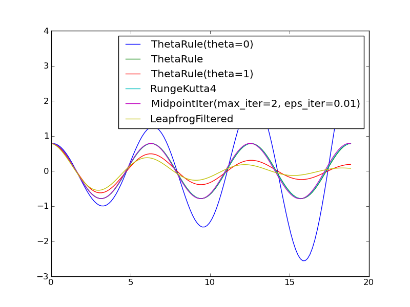
Comparison of methods for solving the ODE system for a pendulum

Make a Subclass of Problem¶

Odespy features a module problems for defining ODE problems. There is a superclass Problem in this module defining what we expect of information about an ODE problem, as well as some convenience functions that are inherited in subclasses. A rough sketch of class Problem is listed here:

class Problem:
    stiff = False    # classification of the problem is stiff or not
    complex_ = False # True if f(u,t) is complex valued
    not_suitable_solvers = []  # list solvers that should be be used
    short_description = ''     # one-line problem description

    def __init__(self):
        pass

    def __contains__(self, attr):
        """Return True if attr is a method in instance self."""

    def terminate(self, u, t, step_number):
        """Default terminate function, always returning False."""
        return False

    def default_parameters(self):
        """
        Compute suitable time_points, atol/rtol, etc. for the
        particular problem. Useful for quick generation of test
        cases, demos, unit tests, etc.
        """
        return {}

    def u_exact(self, t):
        """Implementation of the exact solution."""
        return None

Subclasses of Problem typically implements the constructor, for registering parameters in the ODE and the initial condition, and a method f for defining the right-hand side. For implicit solution method we may provide a method jac returning the Jacobian of $f(u,t)$ with respect to $u$. Some problems may also register an analytical solution in u_exact. Here is an example of implementing the logistic ODE from the section First Example: Logistic Growth:

import odespy

class Logistic(odespy.problems.Problem):
    short_description = "Logistic equation"

    def __init__(self, a, R, A):
        self.a = a
        self.R = R
        self.U0 = A

    def f(self, u, t):
        a, R = self.a, self.R  # short form
        return a*u*(1 - u/R)

    def jac(self, u, t):
        a, R = self.a, self.R  # short form
        return a*(1 - u/R) + a*u*(1 - 1./R)

    def u_exact(self, t):
        a, R, U0 = self.a, self.R, self.U0  # short form
        return R*U0*numpy.exp(a*t)/(R + U0*(numpy.exp(a*t) - 1))

The stiff, complex_, and not_suitable_solvers class variables can just be inherited. Note that u_exact should work for a vector t so numpy versions of mathematical functions must be used.

The initial condition is by convention stored as the attribute U0 in a subclass of Problem, and specified as argument to the constructor.

Here are the typical steps when using such a problem class:

problem = Logistic(a=2, R=1E+5, A=1)
solver = odespy.RK4(problem.f)
solver.set_initial_condition(problem.U0)
u, t = solver.solve(time_points)

The problem class may also feature additional methods:

class MyProblem(odespy.problems.Problem)
    ...
    def constraints(self, u, t):
        """Python function for additional constraints: g(u,t)=0."""

    def define_command_line_arguments(self, parser):
        """
        Initialize an argparse object for reading command-line
        option-value pairs. `parser` is an ``argparse`` object.
        """

    def verify(self, u, t, atol=None, rtol=None):
        """
        Return True if u at time points t coincides with an exact
        solution within the prescribed tolerances. If one of the
        tolerances is None, return max computed error (infinity
        norm). Return None if the solution cannot be verified.
        """

The module odespy.problems contains many predefined ODE problems.

Using Adaptive Methods¶

The solvers used in the previous examples have all employed a constant time step $\Delta t$. Many solvers available through the Odespy interface are adaptive in the sense that $\Delta t$ is adjusted throughout the solution process to meet a prescribed tolerance for the estimated error.

Simple methods such as RK4 apply time steps

dt = time_points[k+1] - time_points[k]

while adaptive methods will use several (smaller) time steps than dt in each dt interval to ensure that the estimated numerical error is smaller than some prescribed tolerance. The estimated numerical error may be a rather crude quantitative measure of the true numerical error (which we do not know since the exact solution of the problem is in general not known).

Some adaptive solvers record the intermediate solutions in each dt interval in arrays self.u_all and self.t_all. Examples include RKFehlberg, Fehlberg, DormandPrince, CashKarp, and BogackiShampine. Other adaptive solvers (Vode, Lsode, Lsoda, RKC, RKF45, etc.) do not give access to intermediate solution steps between the user-given time points, specified in the solver.solve call, and then we only have access to the solution at the user-given time points as returned by this call. One can run if solver.has_u_t_all() to test if the solver.u_all and solver.t_all arrays are available. These are of interest to see how the adaptive strategy works between the user-specified time points.

The Test Problem¶

We consider the ODE problem for testing adaptive solvers:

(1)\[ u' = -\frac{t-c}{s^2} u\]

The exact solution is a Gaussian function,

\[u(t) = \exp{\left(-\frac{1}{2}\left(\frac{t-c}{s}\right)^2\right)}\]

centered around $t=c$ and width characteristic width (“standard deviation”) $s$. The initial condition is taken as the exact $u$ at $t=0$.

Since the Gaussian function is significantly different from zero only in the interval $[c-3s, c+3s]$, one may expect that adaptive methods will efficiently take larger steps when $u$ is almost constant and increase the resolution when $u$ changes substantially in the vicinity of $t=c$. We can test if this is the case with several solvers.

Running Simple Methods¶

Let us first use a simple standard method like the 2nd- and 4th-order Runge-Kutta methods with constant step size. With the former method (RK2), $c=3$, $s=0.5$, and $41$ uniformly distributed points, the discrepancy between the numerical and exact solution in Figure 2nd-order Runge-Kutta method with 41 points for solving :eq:`gaussian:ode:eq` is substantial. Increasing the number of points by a factor of 10 gives a solution much closer to the exact one, and switching to the 4th-order method (RK4) makes the curves visually coincide. The problem is therefore quite straightforward to solve using a sufficient number of points and a higher-order method (for curiosity we can mention that the ForwardEuler method produces a maximum value of 0.98 with 20,000 points and 0.998 with 200,000 points).

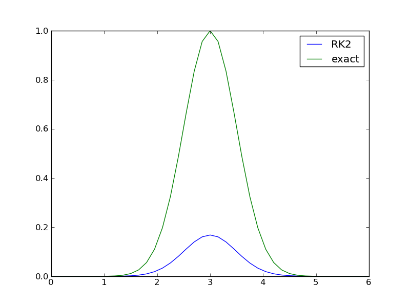
2nd-order Runge-Kutta method with 41 points for solving :eq:`gaussian:ode:eq`

A simple program testing one numerical method goes as follows (gaussian1.py).

import odespy, numpy as np, matplotlib.pyplot as plt

center_point = 3
s = 0.5

problem = odespy.problems.Gaussian0(c=center_point, s=s)

npoints = 41
tp = np.linspace(0, 2*center_point, npoints)

method = odespy.RK4
solver = method(problem.f)
solver.set_initial_condition(problem.U0)

u, t = solver.solve(tp)

method = solver.__class__.__name__
print '%.4f  %s' % (u.max(), method)

if solver.has_u_t_all():
    plt.plot(solver.t_all, solver.u_all, 'bo',
             tp, problem.u_exact(tp))
    print '%s used %d steps (%d specified)' % \
          (method, len(solver.u_all), len(tp))
else:
    plt.plot(tp, solver.u, tp, problem.u_exact(tp))
plt.legend([method, 'exact'])
plt.savefig('tmp.png')
plt.show()

Running the Runge-Kutta-Fehlberg Method¶

One of the most widely used general-purpose, adaptive methods for ODE problems is the Runge-Kutta-Fehlberg method of order (4,5). This method is available in three alternative implementations in Odespy: a direct Python version (RKFehlberg), a specialization of a generalized implementation of explicit adaptive Runge-Kutta methods (Fehlberg), and as a FORTRAN code (RKF45). We can try one of these,

method = odespy.Fehlberg

Figure Adaptive Runge-Kutta-Fehlberg method with 41 points for solving :eq:`gaussian:ode:eq` shows how Fehlberg with 40 intervals produces a solution of reasonable accuracy. The dots show the actual computational points used by the algorithm (113 adaptively selected points in time).

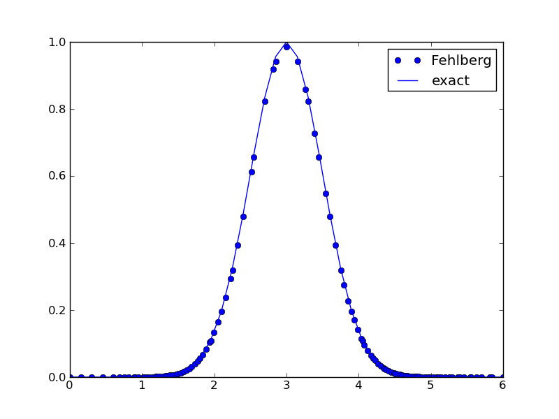
Adaptive Runge-Kutta-Fehlberg method with 41 points for solving :eq:`gaussian:ode:eq`

Adaptive algorithms apply an error estimate based on considering a higher-order method as exact, in this case a method of order 5, and a method of lower order (here 4) as the numerically predicted solution. The user can specify an error tolerance. In the program above we just relied to the default tolerance, which can be printed by

print solver.get()

yielding a list of all optional parameters:

{'f_kwargs': {}, 'f_args': (),
 'max_step': 1.5000000000000036, 'verbose': 0,
 'min_step': 0.0014999999999999946,
 'first_step': 0.14999999999999999,
 'rtol': 1e-06, 'atol': 1e-08,
 'name of f': 'f', 'complex_valued': False,
 'disk_storage': False, 'u_exact': None}

The tolerances involved are of relative and absolute type, i.e.,

estimated_error <= tol = rtol*abs(u) + atol

is the typical test if the solution is accurate enough. For very small u, atol comes into play, while for large u, the relative tolerance rtol dominates.

In this particular example, running RK4 with 113 equally spaced points yields a maximum value of 0.9946, while Fehlberg results in 0.9849. That is, the much simpler and faster RK4 method is also more accurate than the all-round, “reliable” Runge-Kutta-Fehlberg method with an error tolerance of $10^-6$. As we see, the actually error is of the order $10^{-2}$ for the latter method.

We can specify stricter tolerances and also control the minimum allowed step size, min_step, which might be too large to achieve the desired error level (gaussian2.py):

rtol = 1E-6
atol = rtol
min_step = 0.000001

solver = odespy.Fehlberg(problem.f, atol=atol, rtol=rtol,
                         min_step=min_step)

This adjustment does not improve the accuracy. Setting rtol=1E-12 does: the Fehlberg solver then applies 800 points and achieves a maximum value of 1.00004.

Example: Solving a Complex ODE Problem¶

Many of the solvers offered by Odespy can deal with complex-valued ODE problems. Consider

\[u' = iwu,\quad u(0)=1,\]

where $i=\sqrt{-1}$ is the imaginary unit. The right-hand side is implemented as 1j*w*u in Python since Python applies j as the imaginary unit in complex numbers.

Quick Implementation¶

For complex-valued ODEs, i.e., complex-valued right-hand side functions or initial conditions, the argument complex_valued=True must be supplied to the constructor. A complete program reads

def f(u, t):
    return 1j*w*u

import odespy, numpy

w = 2*numpy.pi
solver = odespy.RK4(f, complex_valued=True)
solver.set_initial_condition(1+0j)
u, t = solver.solve(numpy.linspace(0, 6, 101))

The function odespy.list_not_suitable_complex_solvers() returns a list of all the classes in Odespy that are not suitable for complex-valued ODE problems.

Avoiding Callbacks to Python¶

The ODE solvers that are implemented in FORTRAN calls, by default, the user’s Python implementation of $f(u,t)$. Making many calls from FORTRAN to Python may introduce significant overhead and slow down the solution process. When the algorithm is implemented in FORTRAN we should also implement the right-hand side in FORTRAN and call this right-hand side subroutine directly. Odespy offers this possibility.

The idea is that the user writes a FORTRAN subroutine defining $f(u,t)$. Thereafter, f2py is used to make this subroutine callable from Python. If we specify the Python interface to this subroutine as an f_f77 argument to the solver’s constructor, the Odespy class will make sure that no callbacks to the $f(u,t)$ definition go via Python.

The Logistic ODE¶

Here is a minimalistic example involving the logistic ODE from the section First Example: Logistic Growth. The FORTRAN implementation of $f(u,t)$ is more complicated than the Python counterpart. The subroutine has the signature

      subroutine f_f77(neq, t, u, udot)
Cf2py intent(hide) neq
Cf2py intent(out) udot
      integer neq
      double precision t, u, udot
      dimension u(neq), udot(neq)

This means that there are two additional arguments: neq for the number of equations in the ODE system, and udot for the array of $f(u,t)$ that is output from the subroutine.

We write the FORTRAN implementation of $f(u,t)$ in a string:

a = 2
R = 1E+5

f_f77_str = """
      subroutine f_f77(neq, t, u, udot)
Cf2py intent(hide) neq
Cf2py intent(out) udot
      integer neq
      double precision t, u, udot
      dimension u(neq), udot(neq)
      udot(1) = %.3f*u(1)*(1 - u(1)/%.1f)
      return
      end
""" % (a, R)

Observe that we can transfer problem parameters to the FORTRAN subroutine by writing their values directly into the FORTRAN source code. The other alternative would be to transfer the parameters as global (COMMON block) variables to the FORTRAN code, which is technically much more complicated. Also observe that we need to deal with udot and u as arrays even for a scalar ODE.

Using f2py to compile the string into a Python module is automated by the odespy.compile_f77 function:

import odespy
f_f77 = odespy.compile_f77(f_f77_str)

The returned object f_f77 is a callable object that allows the FORTRAN subroutine to be called as udot = f_f77(t, u) from Python. (However, the Odespy solvers will not use f_f77 directly, but rather its function pointer to the FORTRAN subroutine, and transfer this pointer to the FORTRAN solver. The switching between t, u and u, t arguments is taken care of. All necessary steps are automatically done behind the scene.)

The solver can be declared as

solver = odespy.Lsode(f=None, f_f77=f_f77)

Several solvers accept FORTRAN definitions of the right-hand side: Lsode, Lsoda, and the other ODEPACK solvers, RKC, RKF45, Radau5. Look up the documentation of their f_f77 parameter to see exactly what arguments and conventions that the FORTRAN subroutine demand.

The file logistic10.py contains a complete program for solving the logistic ODE with $f(u,t)$ implemented in Fortran.

`odespy`¶

Basic Usage¶

Overview¶

Step 1¶

Step 2¶

Step 3¶

Step 4¶

Step 5¶

Step 6¶

First Example: Logistic Growth¶

Parameters in the Right-Hand Side Function¶

Termination Criterion for the Simulation¶

A Class-Based Implementation¶

Using Other Symbols¶

Example: Solving an ODE System¶

Testing Several Methods¶

Make a Subclass of Problem¶

Using Adaptive Methods¶

The Test Problem¶

Running Simple Methods¶

Running the Runge-Kutta-Fehlberg Method¶

Example: Solving a Complex ODE Problem¶

Quick Implementation¶

Avoiding Callbacks to Python¶

The Logistic ODE¶

Table Of Contents

Previous topic

Next topic

Navigation

odespy¶

Basic Usage¶

Overview¶

Step 1¶

Step 2¶

Step 3¶

Step 4¶

Step 5¶

Step 6¶

First Example: Logistic Growth¶

Parameters in the Right-Hand Side Function¶

Termination Criterion for the Simulation¶

A Class-Based Implementation¶

Using Other Symbols¶

Example: Solving an ODE System¶

Testing Several Methods¶

Make a Subclass of Problem¶

Using Adaptive Methods¶

The Test Problem¶

Running Simple Methods¶

Running the Runge-Kutta-Fehlberg Method¶

Example: Solving a Complex ODE Problem¶

Quick Implementation¶

Avoiding Callbacks to Python¶

The Logistic ODE¶

Table Of Contents

Previous topic

Next topic

Quick search

Navigation

`odespy`¶