The discrete solution
- The numerical solution is a mesh function: \( u_i^n \approx \uex(x_i,t_n) \)
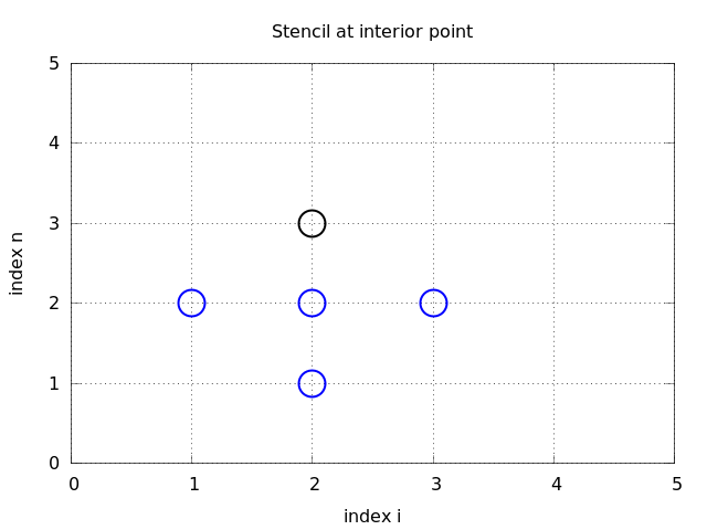
- Finite difference stencil (or scheme): equation for \( u^n_i \) involving neighboring space-time points
Waves on a string can be modeled by the wave equation
$$ \frac{\partial^2 u}{\partial t^2} = c^2 \frac{\partial^2 u}{\partial x^2} $$
\( u(x,t) \) is the displacement of the string
$$
\begin{align}
\frac{\partial^2 u}{\partial t^2} &=
c^2 \frac{\partial^2 u}{\partial x^2}, \quad &x\in (0,L),\ t\in (0,T]
\tag{1}\\
u(x,0) &= I(x), \quad &x\in [0,L]
\tag{2}\\
\frac{\partial}{\partial t}u(x,0) &= 0, \quad &x\in [0,L]
\tag{3}\\
u(0,t) & = 0, \quad &t\in (0,T]
\tag{4}\\
u(L,t) & = 0, \quad &t\in (0,T]
\tag{5}
\end{align}
$$
Rule for number of initial and boundary conditions:
Ooops!
Mesh in time:
$$
\begin{equation}
0 = t_0 < t_1 < t_2 < \cdots < t_{N_t-1} < t_{N_t} = T \tag{6}
\end{equation}
$$
Mesh in space:
$$
\begin{equation}
0 = x_0 < x_1 < x_2 < \cdots < x_{N_x-1} < x_{N_x} = L \tag{7}
\end{equation}
$$
Uniform mesh with constant mesh spacings \( \Delta t \) and \( \Delta x \):
$$
\begin{equation}
x_i = i\Delta x,\ i=0,\ldots,N_x,\quad
t_i = n\Delta t,\ n=0,\ldots,N_t
\tag{8}
\end{equation}
$$
Let the PDE be satisfied at all interior mesh points:
$$
\begin{equation}
\frac{\partial^2}{\partial t^2} u(x_i, t_n) =
c^2\frac{\partial^2}{\partial x^2} u(x_i, t_n),
\tag{9}
\end{equation}
$$
for \( i=1,\ldots,N_x-1 \) and \( n=1,\ldots,N_t-1 \).
For \( n=0 \) we have the initial conditions \( u=I(x) \) and \( u_t=0 \), and at the boundaries \( i=0,N_x \) we have the boundary condition \( u=0 \).
Widely used finite difference formula for the second-order derivative:
$$ \frac{\partial^2}{\partial t^2}u(x_i,t_n)\approx
\frac{u_i^{n+1} - 2u_i^n + u^{n-1}_i}{\Delta t^2}= [D_tD_t u]^n_i$$
and
$$ \frac{\partial^2}{\partial x^2}u(x_i,t_n)\approx
\frac{u_{i+1}^{n} - 2u_i^n + u^{n}_{i-1}}{\Delta x^2} = [D_xD_x u]^n_i
$$
Replace derivatives by differences:
$$
\begin{equation}
\frac{u_i^{n+1} - 2u_i^n + u^{n-1}_i}{\Delta t^2} =
c^2\frac{u_{i+1}^{n} - 2u_i^n + u^{n}_{i-1}}{\Delta x^2},
\tag{10}
\end{equation}
$$
In operator notation:
$$
\begin{equation}
[D_tD_t u = c^2 D_xD_x]^{n}_i
\tag{11}
\end{equation}
$$
$$ [D_{2t} u]^n_i = 0,\quad n=0\quad\Rightarrow\quad
u^{n-1}_i=u^{n+1}_i,\quad i=0,\ldots,N_x$$
The other initial condition \( u(x,0)=I(x) \) can be computed by
$$ u_i^0 = I(x_i),\quad i=0,\ldots,N_x$$
Write out \( [D_tD_t u = c^2 D_xD_x]^{n}_i \) and solve for \( u^{n+1}_i \),
$$
\begin{equation}
u^{n+1}_i = -u^{n-1}_i + 2u^n_i + C^2
\left(u^{n}_{i+1}-2u^{n}_{i} + u^{n}_{i-1}\right)
\tag{12}
\end{equation}
$$
$$
\begin{equation}
C = c\frac{\Delta t}{\Delta x},
\tag{13}
\end{equation}
$$
is known as the (dimensionless) Courant number
There is only one parameter, \( C \), in the discrete model: \( C \) lumps mesh parameters \( \Delta t \) and \( \Delta x \) with the only physical parameter, the wave velocity \( c \). The value \( C \) and the smoothness of \( I(x) \) govern the quality of the numerical solution.
Initial condition:
$$ [D_{2t}u=0]^0_i\quad\Rightarrow\quad u^{-1}_i=u^1_i$$
Insert in stencil \( [D_tD_tu = c^2D_xD_x]^0_i \) to get
$$
\begin{equation}
u_i^1 = u^0_i + \half
C^2\left(u^{n}_{i+1}-2u^{n}_{i} + u^{n}_{i-1}\right)
\tag{14}
\end{equation}
$$
web page or a movie file.
u[i] stores \( u^{n+1}_i \)u_1[i] stores \( u^n_i \)u_2[i] stores \( u^{n-1}_i \)
u is the unknown to be computed (a spatial mesh
function), u_1 denotes the latest computed time level, u_2
corresponds to one time step back in time.
The algorithm only needs to access the three most recent time levels, so we need only three arrays for \( u_i^{n+1} \), \( u_i^n \), and \( u_i^{n-1} \), \( i=0,\ldots,N_x \). Storing all the solutions in a two-dimensional array of size \( (N_x+1)\times (N_t+1) \) would be possible in this simple one-dimensional PDE problem, but not in large 2D problems and not even in small 3D problems.
# Given mesh points as arrays x and t (x[i], t[n])
dx = x[1] - x[0]
dt = t[1] - t[0]
C = c*dt/dx            # Courant number
Nt = len(t)-1
C2 = C**2              # Help variable in the scheme

# Set initial condition u(x,0) = I(x)
for i in range(0, Nx+1):
    u_1[i] = I(x[i])

# Apply special formula for first step, incorporating du/dt=0
for i in range(1, Nx):
    u[i] = u_1[i] + 0.5*C**2(u_1[i+1] - 2*u_1[i] + u_1[i-1])
u[0] = 0;  u[Nx] = 0   # Enforce boundary conditions

# Switch variables before next step
u_2[:], u_1[:] = u_1, u

for n in range(1, Nt):
    # Update all inner mesh points at time t[n+1]
    for i in range(1, Nx):
        u[i] = 2*u_1[i] - u_2[i] + \
               C**2(u_1[i+1] - 2*u_1[i] + u_1[i-1])

    # Insert boundary conditions
    u[0] = 0;  u[Nx] = 0

    # Switch variables before next step
    u_2[:], u_1[:] = u_1, u
Add source term \( f \) and nonzero initial condition \( u_t(x,0) \):
$$
\begin{align}
u_{tt} &= c^2 u_{xx} + f(x,t),
\tag{15}\\
u(x,0) &= I(x), \quad &x\in [0,L]
\tag{16}\\
u_t(x,0) &= V(x), \quad &x\in [0,L]
\tag{17}\\
u(0,t) & = 0, \quad & t>0,
\tag{18}\\
u(L,t) & = 0, \quad &t>0
\tag{19}
\end{align}
$$
$$
\begin{equation}
[D_tD_t u = c^2 D_xD_x + f]^{n}_i
\tag{20}
\end{equation}
$$
Writing out and solving for the unknown \( u^{n+1}_i \):
$$
\begin{equation}
u^{n+1}_i = -u^{n-1}_i + 2u^n_i + C^2
(u^{n}_{i+1}-2u^{n}_{i} + u^{n}_{i-1}) + \Delta t^2 f^n_i
\tag{21}
\end{equation}
$$
Centered difference for \( u_t(x,0) = V(x) \):
$$ [D_{2t}u = V]^0_i\quad\Rightarrow\quad u^{-1}_i = u^{1}_i - 2\Delta t V_i,$$
Inserting this in the stencil (21) for \( n=0 \) leads to
$$
\begin{equation}
u^{1}_i = u^0_i - \Delta t V_i + {\half}
C^2
\left(u^{n}_{i+1}-2u^{n}_{i} + u^{n}_{i-1}\right) + \half\Delta t^2 f^n_i
\tag{22}
\end{equation}
$$
$$
\begin{equation}
\uex(x,y,t)) = A\sin\left(\frac{\pi}{L}x\right)
\cos\left(\frac{\pi}{L}ct\right)
\tag{23}
\end{equation}
$$
$$ \uex(x,t) = x(L-x)\sin t$$
PDE \( u_{tt}=c^2u_{xx}+f \):
$$ -x(L-x)\sin t = -2\sin t + f\quad\Rightarrow f = (2 - x(L-x))\sin t$$
Implied initial conditions:
$$
\begin{align*}
u(x,0) &= I(x) = 0\\
u_t(x,0) &= V(x) = - x(L-x)
\end{align*}
$$
Boundary conditions:
$$ u(0,t) = u(L,t) = 0 $$
Here, choose \( \uex \) such that \( \uex(0,t)=\uex(L,t)=0 \):
$$ \uex (x,t) = x(L-x)(1+{\half}t), $$
Insert in the PDE and find \( f \):
$$ f(x,t)=2(1+t)c^2$$
Initial conditions:
$$ I(x) = x(L-x),\quad V(x)={\half}x(L-x) $$
We want to show that \( \uex \) also solves the discrete equations!
Useful preliminary result:
$$
\begin{align}
\lbrack D_tD_t t^2\rbrack^n &= \frac{t_{n+1}^2 - 2t_n^2 + t_{n-1}^2}{\Delta t^2}
= (n+1)^2 -n^2 + (n-1)^2 = 2
\tag{24}\\
\lbrack D_tD_t t\rbrack^n &= \frac{t_{n+1} - 2t_n + t_{n-1}}{\Delta t^2}
= \frac{((n+1) -n + (n-1))\Delta t}{\Delta t^2} = 0
\tag{25}
\end{align}
$$
Hence,
$$ [D_tD_t \uex]^n_i = x_i(L-x_i)[D_tD_t (1+{\half}t)]^n =
x_i(L-x_i){\half}[D_tD_t t]^n = 0$$
$$
\begin{align*}
\lbrack D_xD_x \uex\rbrack^n_i &=
(1+{\half}t_n)\lbrack D_xD_x (xL-x^2)\rbrack_i =
(1+{\half}t_n)\lbrack LD_xD_x x - D_xD_x x^2\rbrack_i \\
&= -2(1+{\half}t_n)
\end{align*}
$$
Now, \( f^n_i = 2(1+{\half}t_n)c^2 \) and we get
$$ [D_tD_t \uex - c^2D_xD_x\uex - f]^n_i = 0 - c^2(-1)2(1 + {\half}t_n)
+ 2(1+{\half}t_n)c^2 = 0$$
Moreover, \( \uex(x_i,0)=I(x_i) \), \( \partial \uex/\partial t = V(x_i) \) at \( t=0 \), and \( \uex(x_0,t)=\uex(x_{N_x},t)=0 \). Also the modified scheme for the first time step is fulfilled by \( \uex(x_i,t_n) \).
Later we show that the exact solution of the discrete equations can be obtained by \( C=1 \) (!)
def user_action(u, x, t, n):
    # u[i] at spatial mesh points x[i] at time t[n]
    # plot u
    # or store u
import numpy as np

def solver(I, V, f, c, L, dt, C, T, user_action=None):
    """Solve u_tt=c^2*u_xx + f on (0,L)x(0,T]."""
    Nt = int(round(T/dt))
    t = np.linspace(0, Nt*dt, Nt+1)   # Mesh points in time
    dx = dt*c/float(C)
    Nx = int(round(L/dx))
    x = np.linspace(0, L, Nx+1)       # Mesh points in space
    C2 = C**2                      # Help variable in the scheme
    if f is None or f == 0 :
        f = lambda x, t: 0
    if V is None or V == 0:
        V = lambda x: 0

    u   = np.zeros(Nx+1)   # Solution array at new time level
    u_1 = np.zeros(Nx+1)   # Solution at 1 time level back
    u_2 = np.zeros(Nx+1)   # Solution at 2 time levels back

    import time;  t0 = time.clock()  # for measuring CPU time

    # Load initial condition into u_1
    for i in range(0,Nx+1):
        u_1[i] = I(x[i])

    if user_action is not None:
        user_action(u_1, x, t, 0)

    # Special formula for first time step
    n = 0
    for i in range(1, Nx):
        u[i] = u_1[i] + dt*V(x[i]) + \
               0.5*C2*(u_1[i-1] - 2*u_1[i] + u_1[i+1]) + \
               0.5*dt**2*f(x[i], t[n])
    u[0] = 0;  u[Nx] = 0

    if user_action is not None:
        user_action(u, x, t, 1)

    # Switch variables before next step
    u_2[:] = u_1;  u_1[:] = u

    for n in range(1, Nt):
        # Update all inner points at time t[n+1]
        for i in range(1, Nx):
            u[i] = - u_2[i] + 2*u_1[i] + \
                     C2*(u_1[i-1] - 2*u_1[i] + u_1[i+1]) + \
                     dt**2*f(x[i], t[n])

        # Insert boundary conditions
        u[0] = 0;  u[Nx] = 0
        if user_action is not None:
            if user_action(u, x, t, n+1):
                break

        # Switch variables before next step
        u_2[:] = u_1;  u_1[:] = u

    cpu_time = t0 - time.clock()
    return u, x, t, cpu_time
Exact solution of the PDE problem and the discrete equations: \( \uex (x,t) = x(L-x)(1+{\half}t) \)
def test_quadratic():
    """Check that u(x,t)=x(L-x)(1+t/2) is exactly reproduced."""

    def u_exact(x, t):
        return x*(L-x)*(1 + 0.5*t)

    def I(x):
        return u_exact(x, 0)

    def V(x):
        return 0.5*u_exact(x, 0)

    def f(x, t):
        return 2*(1 + 0.5*t)*c**2

    L = 2.5
    c = 1.5
    C = 0.75
    Nx = 6  # Very coarse mesh for this exact test
    dt = C*(L/Nx)/c
    T = 18

    def assert_no_error(u, x, t, n):
        u_e = u_exact(x, t[n])
        diff = np.abs(u - u_e).max()
        tol = 1E-13
        assert diff < tol

    solver(I, V, f, c, L, dt, C, T,
           user_action=assert_no_error)
Make a viz function for animating the curve, with plotting
in a user_action function plot_u:
def viz(
    I, V, f, c, L, dt, C, T,  # PDE paramteres
    umin, umax,               # Interval for u in plots
    animate=True,             # Simulation with animation?
    tool='matplotlib',        # 'matplotlib' or 'scitools'
    solver_function=solver,   # Function with numerical algorithm
    ):
    """Run solver and visualize u at each time level."""

    def plot_u_st(u, x, t, n):
        """user_action function for solver."""
        plt.plot(x, u, 'r-',
                 xlabel='x', ylabel='u',
                 axis=[0, L, umin, umax],
                 title='t=%f' % t[n], show=True)
        # Let the initial condition stay on the screen for 2
        # seconds, else insert a pause of 0.2 s between each plot
        time.sleep(2) if t[n] == 0 else time.sleep(0.2)
        plt.savefig('frame_%04d.png' % n)  # for movie making

    class PlotMatplotlib:
        def __call__(self, u, x, t, n):
            """user_action function for solver."""
            if n == 0:
                plt.ion()
                self.lines = plt.plot(x, u, 'r-')
                plt.xlabel('x');  plt.ylabel('u')
                plt.axis([0, L, umin, umax])
                plt.legend(['t=%f' % t[n]], loc='lower left')
            else:
                self.lines[0].set_ydata(u)
                plt.legend(['t=%f' % t[n]], loc='lower left')
                plt.draw()
            time.sleep(2) if t[n] == 0 else time.sleep(0.2)
            plt.savefig('tmp_%04d.png' % n)  # for movie making

    if tool == 'matplotlib':
        import matplotlib.pyplot as plt
        plot_u = PlotMatplotlib()
    elif tool == 'scitools':
        import scitools.std as plt  # scitools.easyviz interface
        plot_u = plot_u_st
    import time, glob, os

    # Clean up old movie frames
    for filename in glob.glob('tmp_*.png'):
        os.remove(filename)

    # Call solver and do the simulaton
    user_action = plot_u if animate else None
    u, x, t, cpu = solver_function(
        I, V, f, c, L, dt, C, T, user_action)

    # Make video files
    fps = 4  # frames per second
    codec2ext = dict(flv='flv', libx264='mp4', libvpx='webm',
                     libtheora='ogg')  # video formats
    filespec = 'tmp_%04d.png'
    movie_program = 'ffmpeg'  # or 'avconv'
    for codec in codec2ext:
        ext = codec2ext[codec]
        cmd = '%(movie_program)s -r %(fps)d -i %(filespec)s '\
              '-vcodec %(codec)s movie.%(ext)s' % vars()
        os.system(cmd)

    if tool == 'scitools':
        # Make an HTML play for showing the animation in a browser
        plt.movie('tmp_*.png', encoder='html', fps=fps,
                  output_file='movie.html')
    return cpu
Note: plot_u is function inside function and remembers the
local variables in viz (known as a closure).
'something_%04d.png' % frame_counter
Terminal> scitools movie encoder=html output_file=movie.html \
          fps=4 frame_*.png  # web page with a player
Terminal> avconv -r 4 -i frame_%04d.png -c:v flv       movie.flv
Terminal> avconv -r 4 -i frame_%04d.png -c:v libtheora movie.ogg
Terminal> avconv -r 4 -i frame_%04d.png -c:v libx264   movie.mp4
Terminal> avconv -r 4 -i frame_%04d.png -c:v libpvx    movie.webm
%04d) is essential for correct sequence of
frames in something_*.png (Unix alphanumeric sort)frame_*.png files before making a new movie
$$
\begin{equation}
I(x) = \left\lbrace
\begin{array}{ll}
ax/x_0, & x < x_0\\
a(L-x)/(L-x_0), & \hbox{otherwise}
\end{array}\right.
\tag{26}
\end{equation}
$$
Appropriate data:
def guitar(C):
    """Triangular wave (pulled guitar string)."""
    L = 0.75
    x0 = 0.8*L
    a = 0.005
    freq = 440
    wavelength = 2*L
    c = freq*wavelength
    omega = 2*pi*freq
    num_periods = 1
    T = 2*pi/omega*num_periods
    # Choose dt the same as the stability limit for Nx=50
    dt = L/50./c

    def I(x):
        return a*x/x0 if x < x0 else a/(L-x0)*(L-x)

    umin = -1.2*a;  umax = -umin
    cpu = viz(I, 0, 0, c, L, dt, C, T, umin, umax,
              animate=True, tool='scitools')
Program: wave1D_u0.py.
Introduce new \( x \), \( t \), and \( u \) without dimension:
$$ \bar x = \frac{x}{L},\quad \bar t = \frac{c}{L}t,\quad
\bar u = \frac{u}{a}
$$
Insert this in the PDE (with \( f=0 \)) and dropping bars
$$ u_{tt} = u_{xx}$$
Initial condition: set \( a=1 \), \( L=1 \), and \( x_0\in [0,1] \) in (26).
In the code: set a=c=L=1, x0=0.8, and there is no need to calculate with
wavelengths and frequencies to estimate \( c \)!
Just one challenge: determine the period of the waves and an appropriate end time (see the text for details).
numpy) code instead of explicit loopsNext: vectorized loops
n = u.size
for i in range(0, n-1):
    d[i] = u[i+1] - u[i]
numpy code: u[1:n] - u[0:n-1] or just u[1:] - u[:-1]
Newcomers to vectorization are encouraged to choose
a small array u, say with five elements,
and simulate with pen and paper
both the loop version and the vectorized version.
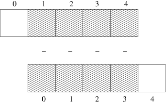
Finite difference schemes basically contains differences between array elements with shifted indices. Consider the updating formula
for i in range(1, n-1):
    u2[i] = u[i-1] - 2*u[i] + u[i+1]
The vectorization consists of replacing the loop by arithmetics on
slices of arrays of length n-2:
u2 = u[:-2] - 2*u[1:-1] + u[2:]
u2 = u[0:n-2] - 2*u[1:n-1] + u[2:n]   # alternative
Note: u2 gets length n-2.
If u2 is already an array of length n, do update on "inner" elements
u2[1:-1]  = u[:-2] - 2*u[1:-1] + u[2:]
u2[1:n-1] = u[0:n-2] - 2*u[1:n-1] + u[2:n]   # alternative
Include a function evaluation too:
def f(x):
    return x**2 + 1

# Scalar version
for i in range(1, n-1):
    u2[i] = u[i-1] - 2*u[i] + u[i+1] + f(x[i])

# Vectorized version
u2[1:-1] = u[:-2] - 2*u[1:-1] + u[2:] + f(x[1:-1])
Scalar loop:
for i in range(1, Nx):
    u[i] = 2*u_1[i] - u_2[i] + \
           C2*(u_1[i-1] - 2*u_1[i] + u_1[i+1])
Vectorized loop:
u[1:-1] = - u_2[1:-1] + 2*u_1[1:-1] + \
          C2*(u_1[:-2] - 2*u_1[1:-1] + u_1[2:])
or
u[1:Nx] = 2*u_1[1:Nx]- u_2[1:Nx] + \
          C2*(u_1[0:Nx-1] - 2*u_1[1:Nx] + u_1[2:Nx+1])
Program: wave1D_u0v.py
def test_quadratic():
    """
    Check the scalar and vectorized versions work for
    a quadratic u(x,t)=x(L-x)(1+t/2) that is exactly reproduced.
    """
    # The following function must work for x as array or scalar
    u_exact = lambda x, t: x*(L - x)*(1 + 0.5*t)
    I = lambda x: u_exact(x, 0)
    V = lambda x: 0.5*u_exact(x, 0)
    # f is a scalar (zeros_like(x) works for scalar x too)
    f = lambda x, t: np.zeros_like(x) + 2*c**2*(1 + 0.5*t)

    L = 2.5
    c = 1.5
    C = 0.75
    Nx = 3  # Very coarse mesh for this exact test
    dt = C*(L/Nx)/c
    T = 18

    def assert_no_error(u, x, t, n):
        u_e = u_exact(x, t[n])
        tol = 1E-13
        diff = np.abs(u - u_e).max()
        assert diff < tol

    solver(I, V, f, c, L, dt, C, T,
           user_action=assert_no_error, version='scalar')
    solver(I, V, f, c, L, dt, C, T,
           user_action=assert_no_error, version='vectorized')
Note:
wave1D_u0v.py for \( N_x \) as 50,100,200,400,800
and measuring the CPU timeMuch bigger improvements for 2D and 3D codes!
$$
\begin{equation}
\frac{\partial u}{\partial n} \equiv \normalvec\cdot\nabla u = 0
\tag{27}
\end{equation}
$$
For a 1D domain \( [0,L] \):
$$
\left.\frac{\partial}{\partial n}\right\vert_{x=L} =
\frac{\partial}{\partial x},\quad
\left.\frac{\partial}{\partial n}\right\vert_{x=0} = -
\frac{\partial}{\partial x}
$$
Boundary condition terminology:
$$
\begin{equation}
\frac{u_{-1}^n - u_1^n}{2\Delta x} = 0
\tag{28}
\end{equation}
$$
$$
\frac{u_{-1}^n - u_1^n}{2\Delta x} = 0
$$
$$
\begin{equation}
u^{n+1}_i = -u^{n-1}_i + 2u^n_i + 2C^2
\left(u^{n}_{i+1}-u^{n}_{i}\right),\quad i=0 \tag{29}
\end{equation}
$$
Discrete equation for computing \( u^3_0 \) in terms of \( u^2_0 \), \( u^1_0 \), and \( u^2_1 \):
Animation in a web page or a movie file.
i = 0
ip1 = i+1
im1 = ip1  # i-1 -> i+1
u[i] = u_1[i] + C2*(u_1[im1] - 2*u_1[i] + u_1[ip1])

i = Nx
im1 = i-1
ip1 = im1  # i+1 -> i-1
u[i] = u_1[i] + C2*(u_1[im1] - 2*u_1[i] + u_1[ip1])

# Or just one loop over all points

for i in range(0, Nx+1):
    ip1 = i+1 if i < Nx else i-1
    im1 = i-1 if i > 0  else i+1
    u[i] = u_1[i] + C2*(u_1[im1] - 2*u_1[i] + u_1[ip1])
Program wave1D_dn0.py
web page or a movie file.
| Notation | Python |
|---|---|
| \( \Ix \) | Ix |
| \( \setb{\Ix} \) | Ix[0] |
| \( \sete{\Ix} \) | Ix[-1] |
| \( \setr{\Ix} \) | Ix[1:] |
| \( \setl{\Ix} \) | Ix[:-1] |
| \( \seti{\Ix} \) | Ix[1:-1] |
Index sets for a problem in the \( x,t \) plane:
$$
\begin{equation}
\Ix = \{0,\ldots,N_x\},\quad \It = \{0,\ldots,N_t\},
\tag{30}
\end{equation}
$$
Implemented in Python as
Ix = range(0, Nx+1)
It = range(0, Nt+1)
A finite difference scheme can with the index set notation be specified as
$$
\begin{align*}
u^{n+1}_i &= -u^{n-1}_i + 2u^n_i + C^2
\left(u^{n}_{i+1}-2u^{n}_{i}+u^{n}_{i-1}\right),
\quad i\in\seti{\Ix},\ n\in\seti{\It}\\
u^{n+1}_i &= 0,
\quad i=\setb{\Ix},\ n\in\seti{\It}\\
u^{n+1}_i &= 0,
\quad i=\sete{\Ix},\ n\in\seti{\It}
\end{align*}
$$
Corresponding implementation:
for n in It[1:-1]:
    for i in Ix[1:-1]:
        u[i] = - u_2[i] + 2*u_1[i] + \
               C2*(u_1[i-1] - 2*u_1[i] + u_1[i+1])
    i = Ix[0];  u[i] = 0
    i = Ix[-1]; u[i] = 0
Program wave1D_dn.py
Add ghost points:
u   = zeros(Nx+3)
u_1 = zeros(Nx+3)
u_2 = zeros(Nx+3)

x = linspace(0, L, Nx+1)  # Mesh points without ghost points
u[-1] will always mean the last element in u0,..,Nx+2
u = zeros(Nx+3)
Ix = range(1, u.shape[0]-1)

# Boundary values: u[Ix[0]], u[Ix[-1]]

# Set initial conditions
for i in Ix:
    u_1[i] = I(x[i-Ix[0]])  # Note i-Ix[0]

# Loop over all physical mesh points
for i in Ix:
    u[i] = - u_2[i] + 2*u_1[i] + \
           C2*(u_1[i-1] - 2*u_1[i] + u_1[i+1])

# Update ghost values
i = Ix[0]          # x=0 boundary
u[i-1] = u[i+1]
i = Ix[-1]         # x=L boundary
u[i+1] = u[i-1]
Program: wave1D_dn0_ghost.py.
Heterogeneous media: varying \( c=c(x) \)
$$
\begin{equation}
\frac{\partial^2 u}{\partial t^2} =
\frac{\partial}{\partial x}\left( q(x)
\frac{\partial u}{\partial x}\right) + f(x,t)
\tag{31}
\end{equation}
$$
This equation sampled at a mesh point \( (x_i,t_n) \):
$$
\frac{\partial^2 }{\partial t^2} u(x_i,t_n) =
\frac{\partial}{\partial x}\left( q(x_i)
\frac{\partial}{\partial x} u(x_i,t_n)\right) + f(x_i,t_n),
$$
The principal idea is to first discretize the outer derivative.
Define
$$ \phi = q(x)
\frac{\partial u}{\partial x}
$$
Then use a centered derivative around \( x=x_i \) for the derivative of \( \phi \):
$$
\left[\frac{\partial\phi}{\partial x}\right]^n_i
\approx \frac{\phi_{i+\half} - \phi_{i-\half}}{\Delta x}
= [D_x\phi]^n_i
$$
Then discretize the inner operators:
$$
\phi_{i+\half} = q_{i+\half}
\left[\frac{\partial u}{\partial x}\right]^n_{i+\half}
\approx q_{i+\half} \frac{u^n_{i+1} - u^n_{i}}{\Delta x}
= [q D_x u]_{i+\half}^n
$$
Similarly,
$$
\phi_{i-\half} = q_{i-\half}
\left[\frac{\partial u}{\partial x}\right]^n_{i-\half}
\approx q_{i-\half} \frac{u^n_{i} - u^n_{i-1}}{\Delta x}
= [q D_x u]_{i-\half}^n
$$
These intermediate results are now combined to
$$
\begin{equation}
\left[
\frac{\partial}{\partial x}\left( q(x)
\frac{\partial u}{\partial x}\right)\right]^n_i
\approx \frac{1}{\Delta x^2}
\left( q_{i+\half} \left({u^n_{i+1} - u^n_{i}}\right)
- q_{i-\half} \left({u^n_{i} - u^n_{i-1}}\right)\right)
\tag{32}
\end{equation}
$$
In operator notation:
$$
\begin{equation}
\left[
\frac{\partial}{\partial x}\left( q(x)
\frac{\partial u}{\partial x}\right)\right]^n_i
\approx [D_xq D_x u]^n_i
\tag{33}
\end{equation}
$$
Many are tempted to use the chain rule on the term \( \frac{\partial}{\partial x}\left( q(x) \frac{\partial u}{\partial x}\right) \), but this is not a good idea!
$$
\begin{align}
q_{i+\half} &\approx
\half\left( q_{i} + q_{i+1}\right) =
[\overline{q}^{x}]_i
\quad &\hbox{(arithmetic mean)}
\tag{34}\\
q_{i+\half} &\approx
2\left( \frac{1}{q_{i}} + \frac{1}{q_{i+1}}\right)^{-1}
\quad &\hbox{(harmonic mean)}
\tag{35}\\
q_{i+\half} &\approx
\left(q_{i}q_{i+1}\right)^{1/2}
\quad &\hbox{(geometric mean)}
\tag{36}
\end{align}
$$
The arithmetic mean in (34) is by far the most used averaging technique.
$$
\begin{equation}
\lbrack D_tD_t u = D_x\overline{q}^{x}D_x u + f\rbrack^{n}_i
\tag{37}
\end{equation}
$$
We clearly see the type of finite differences and averaging!
Write out and solve wrt \( u_i^{n+1} \):
$$
\begin{align}
u^{n+1}_i &= - u_i^{n-1} + 2u_i^n + \left(\frac{\Delta t}{\Delta x}\right)^2\times \nonumber\\
&\quad \left(
\half(q_{i} + q_{i+1})(u_{i+1}^n - u_{i}^n) -
\half(q_{i} + q_{i-1})(u_{i}^n - u_{i-1}^n)\right)
+ \nonumber\\
& \quad \Delta t^2 f^n_i
\tag{38}
\end{align}
$$
Consider \( \partial u/\partial x=0 \) at \( x=L=N_x\Delta x \):
$$ \frac{u_{i+1}^{n} - u_{i-1}^n}{2\Delta x} = 0\quad u_{i+1}^n = u_{i-1}^n,
\quad i=N_x
$$
Insert \( u_{i+1}^n=u_{i-1}^n \) in the stencil (38) for \( i=N_x \) and obtain
$$
u^{n+1}_i \approx
- u_i^{n-1} + 2u_i^n + \left(\frac{\Delta t}{\Delta x}\right)^2
2q_{i}(u_{i-1}^n - u_{i}^n) + \Delta t^2 f^n_i
$$
(We have used \( q_{i+\half} + q_{i-\half}\approx 2q_i \).)
Alternative: assume \( dq/dx=0 \) (simpler).
Assume c[i] holds \( c_i \) the spatial mesh points
for i in range(1, Nx):
    u[i] = - u_2[i] + 2*u_1[i] + \
           C2*(0.5*(q[i] + q[i+1])*(u_1[i+1] - u_1[i])  - \
               0.5*(q[i] + q[i-1])*(u_1[i] - u_1[i-1])) + \
           dt2*f(x[i], t[n])
Here: C2=(dt/dx)**2
Vectorized version:
u[1:-1] = - u_2[1:-1] + 2*u_1[1:-1] + \
          C2*(0.5*(q[1:-1] + q[2:])*(u_1[2:] - u_1[1:-1]) -
              0.5*(q[1:-1] + q[:-2])*(u_1[1:-1] - u_1[:-2])) + \
          dt2*f(x[1:-1], t[n])
Neumann condition \( u_x=0 \): same ideas as in 1D (modified stencil or ghost cells).
$$
\begin{equation}
\varrho(x)\frac{\partial^2 u}{\partial t^2} =
\frac{\partial}{\partial x}\left( q(x)
\frac{\partial u}{\partial x}\right) + f(x,t)
\tag{39}
\end{equation}
$$
A natural scheme is
$$
\begin{equation}
[\varrho D_tD_t u = D_x\overline{q}^xD_x u + f]^n_i
\tag{40}
\end{equation}
$$
Or
$$
\begin{equation}
[D_tD_t u = \varrho^{-1}D_x\overline{q}^xD_x u + f]^n_i
\tag{41}
\end{equation}
$$
No need to average \( \varrho \), just sample at \( i \)
Why do waves die out?
Simplest damping model (for physical behavior, see demo):
$$
\begin{equation}
\frac{\partial^2 u}{\partial t^2} + \color{red}{b\frac{\partial u}{\partial t}}
= c^2\frac{\partial^2 u}{\partial x^2} + f(x,t),
\tag{42}
\end{equation}
$$
\( b \geq 0 \): prescribed damping coefficient.
Discretization via centered differences to ensure \( \Oof{\Delta t^2} \) error:
$$
\begin{equation}
[D_tD_t u + bD_{2t}u = c^2D_xD_x u + f]^n_i
\tag{43}
\end{equation}
$$
Need special formula for \( u^1_i \) + special stencil (or ghost cells) for Neumann conditions.
The program wave1D_dn_vc.py solves a fairly general 1D wave equation:
$$
\begin{align}
u_{tt} &= (c^2(x)u_x)_x + f(x,t),\quad &x\in (0,L),\ t\in (0,T]
\tag{44}\\
u(x,0) &= I(x),\quad &x\in [0,L]
\tag{45}\\
u_t(x,0) &= V(t),\quad &x\in [0,L]
\tag{46}\\
u(0,t) &= U_0(t)\hbox{ or } u_x(0,t)=0,\quad &t\in (0,T]
\tag{47}\\
u(L,t) &= U_L(t)\hbox{ or } u_x(L,t)=0,\quad &t\in (0,T]
\tag{48}
\end{align}
$$
Can be adapted to many needs.
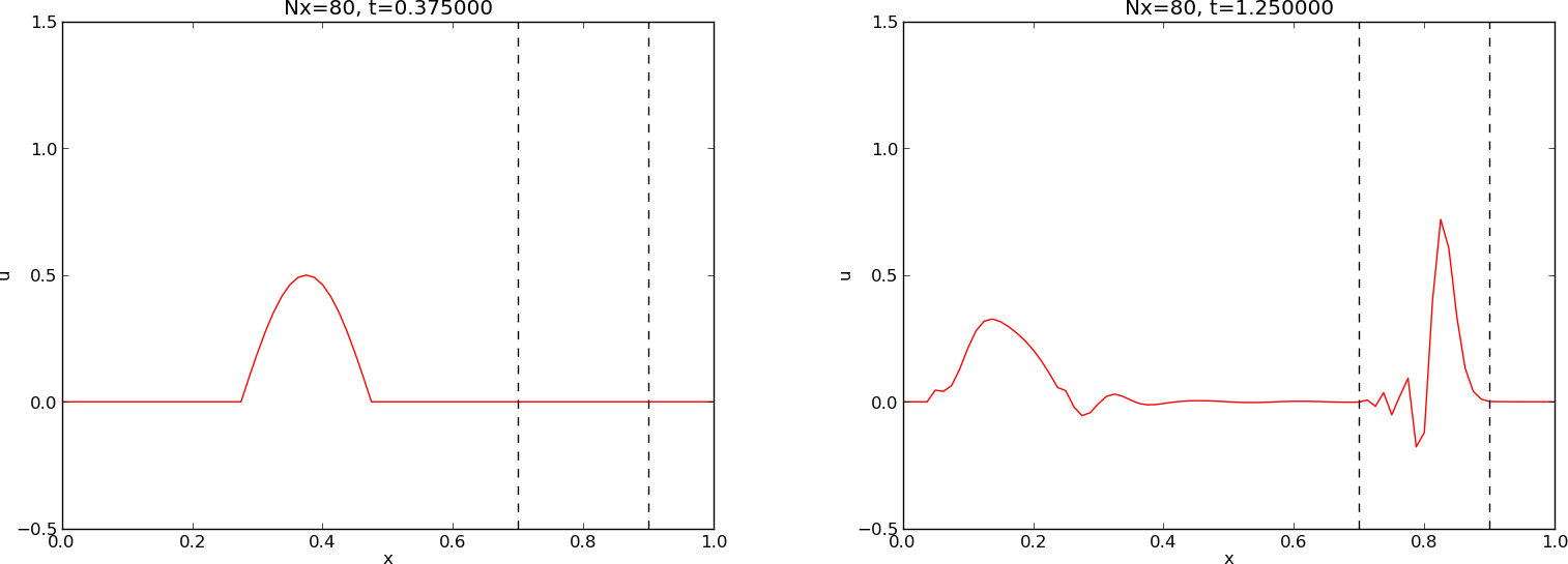
The function pulse in wave1D_dn_vc.py offers four
initial conditions:
gaussian)Can locate the initial pulse at \( x=0 \) or in the middle
>>> import wave1D_dn_vc as w
>>> w.pulse(loc='left', pulse_tp='cosinehat', Nx=50, every_frame=10)
Constant wave velocity \( c \):
$$
\begin{equation}
\frac{\partial^2 u}{\partial t^2} = c^2\nabla^2 u\hbox{ for }\xpoint\in\Omega\subset\Real^d,\ t\in (0,T]
\tag{49}
\end{equation}
$$
Variable wave velocity:
$$
\begin{equation}
\varrho\frac{\partial^2 u}{\partial t^2} = \nabla\cdot (q\nabla u) + f\hbox{ for }\xpoint\in\Omega\subset\Real^d,\ t\in (0,T]
\tag{50}
\end{equation}
$$
3D, constant \( c \):
$$
\begin{equation*} \nabla^2 u = \frac{\partial^2 u}{\partial x^2} +
\frac{\partial^2 u}{\partial y^2} + \frac{\partial^2 u}{\partial z^2}
\end{equation*}
$$
2D, variable \( c \):
$$
\begin{equation}
\varrho(x,y)
\frac{\partial^2 u}{\partial t^2} =
\frac{\partial}{\partial x}\left( q(x,y)
\frac{\partial u}{\partial x}\right)
+
\frac{\partial}{\partial y}\left( q(x,y)
\frac{\partial u}{\partial y}\right)
+ f(x,y,t)
\tag{51}
\end{equation}
$$
Compact notation:
$$
\begin{align}
u_{tt} &= c^2(u_{xx} + u_{yy} + u_{zz}) + f,
\tag{52}\\
\varrho u_{tt} &= (q u_x)_x + (q u_z)_z + (q u_z)_z + f
\tag{53}
\end{align}
$$
We need one boundary condition at each point on \( \partial\Omega \):
PDEs with second-order time derivative need two initial conditions:
$$
[D_tD_t u = c^2(D_xD_x u + D_yD_yu) + f]^n_{i,j,k},
$$
Written out in detail:
$$
\begin{align*}
\frac{u^{n+1}_{i,j} - 2u^{n}_{i,j} + u^{n-1}_{i,j}}{\Delta t^2}
&= c^2
\frac{u^{n}_{i+1,j} - 2u^{n}_{i,j} + u^{n}_{i-1,j}}{\Delta x^2}
+ \nonumber\\
&\quad c^2\frac{u^{n}_{i,j+1} - 2u^{n}_{i,j} + u^{n}_{i,j-1}}{\Delta y^2}
+ f^n_{i,j},
\end{align*}
$$
\( u^{n-1}_{i,j} \) and \( u^n_{i,j} \) are known, solve for \( u^{n+1}_{i,j} \):
$$ u^{n+1}_{i,j} = 2u^n_{i,j} + u^{n-1}_{i,j} + c^2\Delta t^2[D_xD_x u + D_yD_y u]^n_{i,j}$$
$$ [D_{2t}u = V]^0_{i,j}\quad\Rightarrow\quad u^{-1}_{i,j} = u^1_{i,j} - 2\Delta t V_{i,j}
$$
$$ u^{n+1}_{i,j} = u^n_{i,j} -\Delta t V_{i,j} + {\half}
c^2\Delta t^2[D_xD_x u + D_yD_y u]^n_{i,j}$$
3D wave equation:
$$ \varrho u_{tt} = (qu_x)_x + (qu_y)_y + (qu_z)_z + f(x,y,z,t) $$
Just apply the 1D discretization for each term:
$$
\begin{equation}
[\varrho D_tD_t u = (D_x\overline{q}^x D_x u +
D_y\overline{q}^y D_yu + D_z\overline{q}^z D_z u) + f]^n_{i,j,k}
\tag{54}
\end{equation}
$$
Need special formula for \( u^1_{i,j,k} \) (use \( [D_{2t}u=V]^0 \) and stencil for \( n=0 \)).
Written out:
$$
\begin{align*}
u^{n+1}_{i,j,k} &= - u^{n-1}_{i,j,k} + 2u^{n}_{i,j,k} \\
&+ \frac{\Delta t^2}{\varrho_{i,j,k}}\frac{1}{\Delta x^2} ( \half(q_{i,j,k} + q_{i+1,j,k})(u^{n}_{i+1,j,k} - u^{n}_{i,j,k}) - \\
&\qquad\quad \half(q_{i-1,j,k} + q_{i,j,k})(u^{n}_{i,j,k} - u^{n}_{i-1,j,k})) \\
&+ \frac{\Delta t^2}{\varrho_{i,j,k}}\frac{1}{\Delta y^2} ( \half(q_{i,j,k} + q_{i,j+1,k})(u^{n}_{i,j+1,k} - u^{n}_{i,j,k}) - \\
&\qquad\quad\half(q_{i,j-1,k} + q_{i,j,k})(u^{n}_{i,j,k} - u^{n}_{i,j-1,k})) \\
&+ \frac{\Delta t^2}{\varrho_{i,j,k}}\frac{1}{\Delta z^2} ( \half(q_{i,j,k} + q_{i,j,k+1})(u^{n}_{i,j,k+1} - u^{n}_{i,j,k}) -\\
&\qquad\quad \half(q_{i,j,k-1} + q_{i,j,k})(u^{n}_{i,j,k} - u^{n}_{i,j,k-1})) + \\
&+\qquad \Delta t^2 f^n_{i,j,k}
\end{align*}
$$
Use ideas from 1D! Example: \( \frac{\partial u}{\partial n}=0 \) at \( y=0 \), \( \frac{\partial u}{\partial n} = -\frac{\partial u}{\partial y} \)
Boundary condition discretization:
$$ [-D_{2y} u = 0]^n_{i,0}\quad\Rightarrow\quad \frac{u^n_{i,1}-u^n_{i,-1}}{2\Delta y} = 0,\ i\in\Ix
$$
Insert \( u^n_{i,-1}=u^n_{i,1} \) in the stencil for \( u^{n+1}_{i,j=0} \) to obtain a modified stencil on the boundary.
Pattern: use interior stencil also on the bundary, but replace \( j-1 \) by \( j+1 \)
Alternative: use ghost cells and ghost values
$$
\begin{align}
u_{tt} &= c^2(u_{xx} + u_{yy}) + f(x,y,t),\quad &(x,y)\in \Omega,\ t\in (0,T]
\tag{55}\\
u(x,y,0) &= I(x,y),\quad &(x,y)\in\Omega
\tag{56}\\
u_t(x,y,0) &= V(x,y),\quad &(x,y)\in\Omega
\tag{57}\\
u &= 0,\quad &(x,y)\in\partial\Omega,\ t\in (0,T]
\tag{58}
\end{align}
$$
\( \Omega = [0,L_x]\times [0,L_y] \)
Discretization:
$$ [D_t D_t u = c^2(D_xD_x u + D_yD_y u) + f]^n_{i,j},
$$
Program: wave2D_u0.py
def solver(I, V, f, c, Lx, Ly, Nx, Ny, dt, T,
           user_action=None, version='scalar'):
Mesh:
x = linspace(0, Lx, Nx+1)                  # mesh points in x dir
y = linspace(0, Ly, Ny+1)                  # mesh points in y dir
dx = x[1] - x[0]
dy = y[1] - y[0]
Nt = int(round(T/float(dt)))
t = linspace(0, N*dt, N+1)                 # mesh points in time
Cx2 = (c*dt/dx)**2;  Cy2 = (c*dt/dy)**2    # help variables
dt2 = dt**2
Store \( u^{n+1}_{i,j} \), \( u^{n}_{i,j} \), and \( u^{n-1}_{i,j} \) in three two-dimensional arrays:
u   = zeros((Nx+1,Ny+1))   # solution array
u_1 = zeros((Nx+1,Ny+1))   # solution at t-dt
u_2 = zeros((Nx+1,Ny+1))   # solution at t-2*dt
\( u^{n+1}_{i,j} \) corresponds to u[i,j], etc.
Ix = range(0, u.shape[0])
Iy = range(0, u.shape[1])
It = range(0, t.shape[0])

for i in Ix:
    for j in Iy:
        u_1[i,j] = I(x[i], y[j])

if user_action is not None:
    user_action(u_1, x, xv, y, yv, t, 0)
Arguments xv and yv: for vectorized computations
def advance_scalar(u, u_1, u_2, f, x, y, t, n, Cx2, Cy2, dt2,
                   V=None, step1=False):
    Ix = range(0, u.shape[0]);  Iy = range(0, u.shape[1])
    if step1:
        dt = sqrt(dt2)  # save
        Cx2 = 0.5*Cx2;  Cy2 = 0.5*Cy2; dt2 = 0.5*dt2  # redefine
        D1 = 1;  D2 = 0
    else:
        D1 = 2;  D2 = 1
    for i in Ix[1:-1]:
        for j in Iy[1:-1]:
            u_xx = u_1[i-1,j] - 2*u_1[i,j] + u_1[i+1,j]
            u_yy = u_1[i,j-1] - 2*u_1[i,j] + u_1[i,j+1]
            u[i,j] = D1*u_1[i,j] - D2*u_2[i,j] + \
                     Cx2*u_xx + Cy2*u_yy + dt2*f(x[i], y[j], t[n])
            if step1:
                u[i,j] += dt*V(x[i], y[j])
    # Boundary condition u=0
    j = Iy[0]
    for i in Ix: u[i,j] = 0
    j = Iy[-1]
    for i in Ix: u[i,j] = 0
    i = Ix[0]
    for j in Iy: u[i,j] = 0
    i = Ix[-1]
    for j in Iy: u[i,j] = 0
    return u
D1 and D2: allow advance_scalar to be used also for \( u^1_{i,j} \):
u = advance_scalar(u, u_1, u_2, f, x, y, t,
                   n, 0.5*Cx2, 0.5*Cy2, 0.5*dt2, D1=1, D2=0)
Mesh with \( 30\times 30 \) cells: vectorization reduces the CPU time by a factor of 70 (!).
Need special coordinate arrays xv and yv such that \( I(x,y) \)
and \( f(x,y,t) \) can be vectorized:
from numpy import newaxis
xv = x[:,newaxis]
yv = y[newaxis,:]

u_1[:,:] = I(xv, yv)
f_a[:,:] = f(xv, yv, t)
def advance_vectorized(u, u_1, u_2, f_a, Cx2, Cy2, dt2,
                       V=None, step1=False):
    if step1:
        dt = sqrt(dt2)  # save
        Cx2 = 0.5*Cx2;  Cy2 = 0.5*Cy2; dt2 = 0.5*dt2  # redefine
        D1 = 1;  D2 = 0
    else:
        D1 = 2;  D2 = 1
    u_xx = u_1[:-2,1:-1] - 2*u_1[1:-1,1:-1] + u_1[2:,1:-1]
    u_yy = u_1[1:-1,:-2] - 2*u_1[1:-1,1:-1] + u_1[1:-1,2:]
    u[1:-1,1:-1] = D1*u_1[1:-1,1:-1] - D2*u_2[1:-1,1:-1] + \
                   Cx2*u_xx + Cy2*u_yy + dt2*f_a[1:-1,1:-1]
    if step1:
        u[1:-1,1:-1] += dt*V[1:-1, 1:-1]
    # Boundary condition u=0
    j = 0
    u[:,j] = 0
    j = u.shape[1]-1
    u[:,j] = 0
    i = 0
    u[i,:] = 0
    i = u.shape[0]-1
    u[i,:] = 0
    return u

def quadratic(Nx, Ny, version):
    """Exact discrete solution of the scheme."""

    def exact_solution(x, y, t):
        return x*(Lx - x)*y*(Ly - y)*(1 + 0.5*t)

    def I(x, y):
        return exact_solution(x, y, 0)

    def V(x, y):
        return 0.5*exact_solution(x, y, 0)

    def f(x, y, t):
        return 2*c**2*(1 + 0.5*t)*(y*(Ly - y) + x*(Lx - x))

    Lx = 5;  Ly = 2
    c = 1.5
    dt = -1 # use longest possible steps
    T = 18

    def assert_no_error(u, x, xv, y, yv, t, n):
        u_e = exact_solution(xv, yv, t[n])
        diff = abs(u - u_e).max()
        tol = 1E-12
        msg = 'diff=%g, step %d, time=%g' % (diff, n, t[n])
        assert diff < tol, msg

    new_dt, cpu = solver(
        I, V, f, c, Lx, Ly, Nx, Ny, dt, T,
        user_action=assert_no_error, version=version)
    return new_dt, cpu


def test_quadratic():
    # Test a series of meshes where Nx > Ny and Nx < Ny
    versions = 'scalar', 'vectorized', 'cython', 'f77', 'c_cy', 'c_f2py'
    for Nx in range(2, 6, 2):
        for Ny in range(2, 6, 2):
            for version in versions:
                print 'testing', version, 'for %dx%d mesh' % (Nx, Ny)
                quadratic(Nx, Ny, version)

def run_efficiency(nrefinements=4):
    def I(x, y):
        return sin(pi*x/Lx)*sin(pi*y/Ly)

    Lx = 10;  Ly = 10
    c = 1.5
    T = 100
    versions = ['scalar', 'vectorized', 'cython', 'f77',
               'c_f2py', 'c_cy']
    print ' '*15, ''.join(['%-13s' % v for v in versions])
    for Nx in 15, 30, 60, 120:
        cpu = {}
        for version in versions:
            dt, cpu_ = solver(I, None, None, c, Lx, Ly, Nx, Nx,
                              -1, T, user_action=None,
                              version=version)
            cpu[version] = cpu_
        cpu_min = min(list(cpu.values()))
        if cpu_min < 1E-6:
            print 'Ignored %dx%d grid (too small execution time)' \
                  % (Nx, Nx)
        else:
            cpu = {version: cpu[version]/cpu_min for version in cpu}
            print '%-15s' % '%dx%d' % (Nx, Nx),
            print ''.join(['%13.1f' % cpu[version] for version in versions])

def gaussian(plot_method=2, version='vectorized', save_plot=True):
    """
    Initial Gaussian bell in the middle of the domain.
    plot_method=1 applies mesh function, =2 means surf, =0 means no plot.
    """
    # Clean up plot files
    for name in glob('tmp_*.png'):
        os.remove(name)

    Lx = 10
    Ly = 10
    c = 1.0

    def I(x, y):
        """Gaussian peak at (Lx/2, Ly/2)."""
        return exp(-0.5*(x-Lx/2.0)**2 - 0.5*(y-Ly/2.0)**2)

    if plot_method == 3:
        from mpl_toolkits.mplot3d import axes3d
        import matplotlib.pyplot as plt
        from matplotlib import cm
        plt.ion()
        fig = plt.figure()
        u_surf = None

    def plot_u(u, x, xv, y, yv, t, n):
        if t[n] == 0:
            time.sleep(2)
        if plot_method == 1:
            mesh(x, y, u, title='t=%g' % t[n], zlim=[-1,1],
                 caxis=[-1,1])
        elif plot_method == 2:
            surfc(xv, yv, u, title='t=%g' % t[n], zlim=[-1, 1],
                  colorbar=True, colormap=hot(), caxis=[-1,1],
                  shading='flat')
        elif plot_method == 3:
            print 'Experimental 3D matplotlib...under development...'
            #plt.clf()
            ax = fig.add_subplot(111, projection='3d')
            u_surf = ax.plot_surface(xv, yv, u, alpha=0.3)
            #ax.contourf(xv, yv, u, zdir='z', offset=-100, cmap=cm.coolwarm)
            #ax.set_zlim(-1, 1)
            # Remove old surface before drawing
            if u_surf is not None:
                ax.collections.remove(u_surf)
            plt.draw()
            time.sleep(1)
        if plot_method > 0:
            time.sleep(0) # pause between frames
            if save_plot:
                filename = 'tmp_%04d.png' % n
                savefig(filename)  # time consuming!

    Nx = 40; Ny = 40; T = 20
    dt, cpu = solver(I, None, None, c, Lx, Ly, Nx, Ny, -1, T,
                     user_action=plot_u, version=version)


if __name__ == '__main__':
    test_quadratic()
Manufactured solution:
$$
\begin{equation}
\uex(x,y,t) = x(L_x-x)y(L_y-y)(1+{\half}t)
\tag{59}
\end{equation}
$$
Requires \( f=2c^2(1+{\half}t)(y(L_y-y) + x(L_x-x)) \).
This \( \uex \) is ideal because it also solves the discrete equations!
$$
\begin{align*}
[D_xD_x \uex]^n_{i,j} &= [y(L_y-y)(1+{\half}t) D_xD_x x(L_x-x)]^n_{i,j}\\
&= y_j(L_y-y_j)(1+{\half}t_n)2
\end{align*}
$$
$$
\begin{equation*} \frac{\partial^2 u}{\partial t^2} =
c^2 \frac{\partial^2 u}{\partial x^2}
\end{equation*}
$$
Solutions:
$$
u(x,t) = g_R(x-ct) + g_L(x+ct)
$$
If \( u(x,0)=I(x) \) and \( u_t(x,0)=0 \):
$$
u(x,t) = \half I(x-ct) + \half I(x+ct)
$$
Two waves: one traveling to the right and one to the left
A wave propagates perfectly (\( C=1 \)) and hits a medium with 1/4 of the wave velocity (\( C=0.25 \)). A part of the wave is reflected and the rest is transmitted.
Build \( I(x) \) of wave components \( e^{ikx} = \cos kx + i\sin kx \):
$$
I(x) \approx \sum_{k\in K} b_k e^{ikx}
$$
Since \( u(x,t)=\half I(x-ct) + \half I(x+ct) \), the exact solution is
$$
u(x,t) = \half \sum_{k\in K} b_k e^{ik(x - ct)}
+ \half \sum_{k\in K} b_k e^{ik(x + ct)}
$$
Our interest: one component \( e^{i(kx -\omega t)} \), \( \omega = kc \)
Idea: a similar discrete \( u^n_q = e^{i(kx_q - \tilde\omega t_n)} \) solution (corresponding to the exact \( e^{i(kx - \omega t)} \)) solves
$$
[D_tD_t u = c^2 D_xD_x u]^n_q
$$
Note: we expect numerical frequency \( \tilde\omega\neq\omega \)
$$
[D_tD_t e^{i\omega t}]^n = -\frac{4}{\Delta t^2}\sin^2\left(
\frac{\omega\Delta t}{2}\right)e^{i\omega n\Delta t}
$$
By \( \omega\rightarrow k \), \( t\rightarrow x \), \( n\rightarrow q \)) it follows that
$$
[D_xD_x e^{ikx}]_q = -\frac{4}{\Delta x^2}\sin^2\left(
\frac{k\Delta x}{2}\right)e^{ikq\Delta x}
$$
Inserting a basic wave component \( u=e^{i(kx_q-\tilde\omega t_n)} \) in the scheme requires computation of
$$
\begin{align*}
\lbrack D_tD_t e^{ikx}e^{-i\tilde\omega t}\rbrack^n_q &= \lbrack D_tD_t e^{-i\tilde\omega t}\rbrack^ne^{ikq\Delta x}\nonumber\\ &= -\frac{4}{\Delta t^2}\sin^2\left(
\frac{\tilde\omega\Delta t}{2}\right)e^{-i\tilde\omega n\Delta t}e^{ikq\Delta x}\\
\lbrack D_xD_x e^{ikx}e^{-i\tilde\omega t}\rbrack^n_q &= \lbrack D_xD_x e^{ikx}\rbrack_q e^{-i\tilde\omega n\Delta t}\nonumber\\ &= -\frac{4}{\Delta x^2}\sin^2\left(
\frac{k\Delta x}{2}\right)e^{ikq\Delta x}e^{-i\tilde\omega n\Delta t}
\end{align*}
$$
The complete scheme,
$$
\lbrack D_tD_t e^{ikx}e^{-i\tilde\omega t} = c^2D_xD_x e^{ikx}e^{-i\tilde\omega t}\rbrack^n_q
$$
leads to an equation for \( \tilde\omega \) (which can readily be solved):
$$
\sin^2\left(\frac{\tilde\omega\Delta t}{2}\right)
= C^2\sin^2\left(\frac{k\Delta x}{2}\right),\quad C = \frac{c\Delta t}{\Delta x}
\mbox{ (Courant number)}
$$
Taking the square root:
$$
\sin\left(\frac{\tilde\omega\Delta t}{2}\right)
= C\sin\left(\frac{k\Delta x}{2}\right)
$$
Can easily solve for an explicit formula for \( \tilde\omega \):
$$
\tilde\omega = \frac{2}{\Delta t}
\sin^{-1}\left( C\sin\left(\frac{k\Delta x}{2}\right)\right)
$$
Note:
$$
r(C, p) = \frac{\tilde c}{c} =
\frac{2}{kc\Delta t} \sin^{-1}(C\sin p) =
\frac{2}{kC\Delta x} \sin^{-1}(C\sin p) =
\frac{1}{Cp}{\sin}^{-1}\left(C\sin p\right)
$$
Can plot \( r(C,p) \) for \( p\in (0,\pi/2] \), \( C\in (0,1] \)
def r(C, p):
    return 1/(C*p)*asin(C*sin(p))
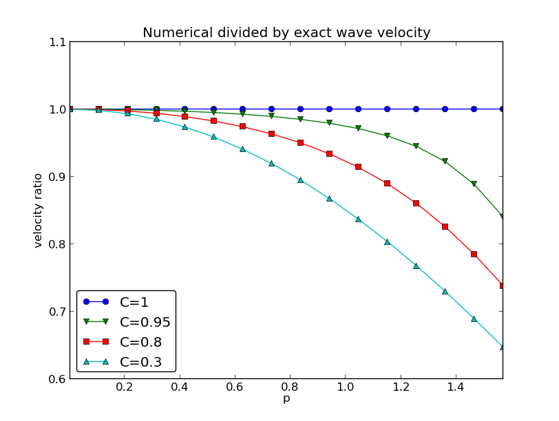
Note: the shortest waves have the largest error, and short waves move too slowly.
For small \( p \), Taylor expand \( \tilde\omega \) as polynomial in \( p \):
>>> C, p = symbols('C p')
>>> rs = r(C, p).series(p, 0, 7)
>>> print rs
1 - p**2/6 + p**4/120 - p**6/5040 + C**2*p**2/6 -
C**2*p**4/12 + 13*C**2*p**6/720 + 3*C**4*p**4/40 -
C**4*p**6/16 + 5*C**6*p**6/112 + O(p**7)

>>> # Drop the remainder O(...) term
>>> rs = rs.removeO()
>>> # Factorize each term
>>> rs = [factor(term) for term in rs.as_ordered_terms()]
>>> rs = sum(rs)
>>> print rs
p**6*(C - 1)*(C + 1)*(225*C**4 - 90*C**2 + 1)/5040 +
p**4*(C - 1)*(C + 1)*(3*C - 1)*(3*C + 1)/120 +
p**2*(C - 1)*(C + 1)/6 + 1
Leading error term is \( \frac{1}{6}(C^2-1)p^2 \) or
$$
\frac{1}{6}\left(\frac{k\Delta x}{2}\right)^2(C^2-1)
= \frac{k^2}{24}\left( c^2\Delta t^2 - \Delta x^2\right) =
\Oof{\Delta t^2, \Delta x^2}
$$
Smooth wave, few short waves (large \( k \)) in \( I(x) \):
Not so smooth wave, significant short waves (large \( k \)) in \( I(x) \):
$$
\sin\left(\frac{\tilde\omega\Delta t}{2}\right)
= C\sin\left(\frac{k\Delta x}{2}\right)
$$
Stability criterion:
$$
C = \frac{c\Delta t}{\Delta x} \leq 1
$$
Recall that right-hand side is in \( [-C,C] \). Then \( C>1 \) means
$$
\underbrace{\sin\left(\frac{\tilde\omega\Delta t}{2}\right)}_{>1} = C\sin\left(\frac{k\Delta x}{2}\right)
$$
$$ u(x,y,t) = g(k_xx + k_yy - \omega t) $$
is a typically solution of
$$ u_{tt} = c^2(u_{xx} + u_{yy}) $$
Can build solutions by adding complex Fourier components of the form
$$
e^{i(k_xx + k_yy - \omega t)}
$$
$$
\lbrack D_tD_t u = c^2(D_xD_x u + D_yD_y u)\rbrack^n_{q,r}
$$
This equation admits a Fourier component
$$
u^n_{q,r} = e^{i(k_x q\Delta x + k_y r\Delta y -
\tilde\omega n\Delta t)}
$$
Inserting the Fourier component into the dicrete 2D wave equation, and using formulas from the 1D analysis:
$$
\sin^2\left(\frac{\tilde\omega\Delta t}{2}\right)
= C_x^2\sin^2 p_x
+ C_y^2\sin^2 p_y
$$
where
$$ C_x = \frac{c\Delta t}{\Delta x},\quad
C_y = \frac{c\Delta t}{\Delta y}, \quad
p_x = \frac{k_x\Delta x}{2},\quad
p_y = \frac{k_y\Delta y}{2}
$$
Ensuring real-valued \( \tilde\omega \) requires
$$
C_x^2 + C_y^2 \leq 1
$$
or
$$
\Delta t \leq \frac{1}{c} \left( \frac{1}{\Delta x^2} +
\frac{1}{\Delta y^2}\right)^{-\halfi}
$$
$$
\Delta t \leq \frac{1}{c}\left( \frac{1}{\Delta x^2} +
\frac{1}{\Delta y^2} + \frac{1}{\Delta z^2}\right)^{-\halfi}
$$
For \( c^2=c^2(\xpoint) \) we must use the worst-case value \( \bar c = \sqrt{\max_{\xpoint\in\Omega} c^2(\xpoint)} \) and a safety factor \( \beta\leq 1 \):
$$
\Delta t \leq \beta \frac{1}{\bar c}
\left( \frac{1}{\Delta x^2} +
\frac{1}{\Delta y^2} + \frac{1}{\Delta z^2}\right)^{-\halfi}
$$
$$
\tilde\omega = \frac{2}{\Delta t}\sin^{-1}\left(
\left( C_x^2\sin^2 p_x + C_y^2\sin^ p_y\right)^\half\right)
$$
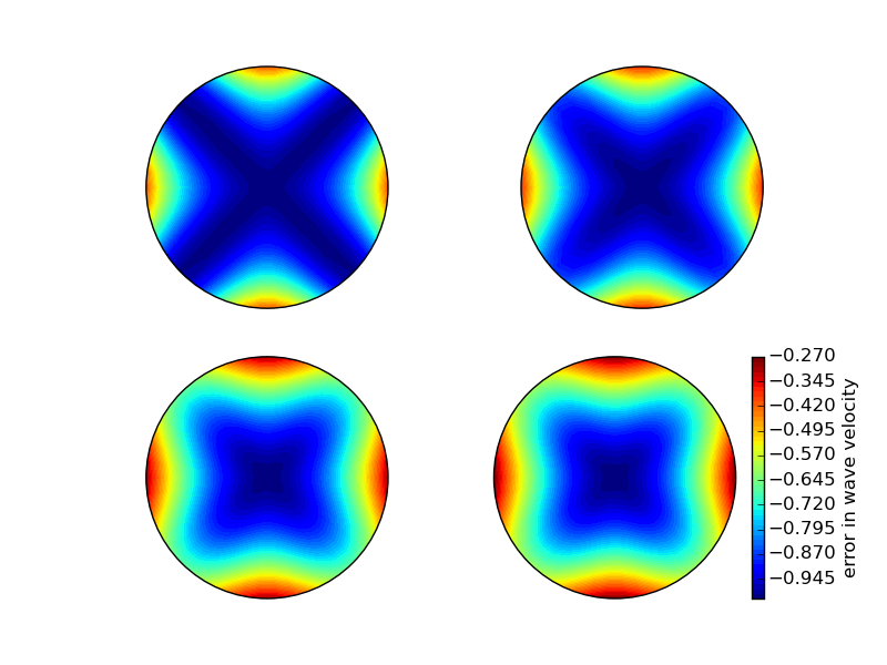
For visualization, introduce \( k=\sqrt{k_x^2+k_y^2} \) and \( \theta \) such that
$$ k_x = k\sin\theta,\quad k_y=k\cos\theta,
\quad p_x=\half kh\cos\theta,\quad p_y=\half kh\sin\theta$$
Also: \( \Delta x=\Delta y=h \). Then \( C_x=C_y=c\Delta t/h\equiv C \).
Now \( \tilde\omega \) depends on
$$ \frac{\tilde c}{c} = \frac{1}{Ckh}
\sin^{-1}\left(C\left(\sin^2 ({\half}kh\cos\theta)
+ \sin^2({\half}kh\sin\theta) \right)^\half\right)
$$
Can make color contour plots of \( 1-\tilde c/c \) in polar coordinates with \( \theta \) as the angular coordinate and \( kh \) as the radial coordinate.