A simple vibration problem
A centered finite difference scheme; step 1 and 2
A centered finite difference scheme; step 3
A centered finite difference scheme; step 4
Computing the first step
The computational algorithm
Operator notation; ODE
Operator notation; initial condition
Computing \( u^{\prime} \)
Implementation
Core algorithm
Plotting
Main program
User interface: command line
Running the program
Verification
First steps for testing and debugging
Checking convergence rates
Implementational details
Unit test for the convergence rate
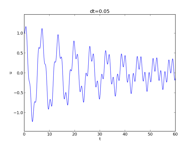
Long time simulations
Effect of the time step on long simulations
Using a moving plot window
Long time simulations visualized with aid of Bokeh: coupled panning of multiple graphs
How does Bokeh plotting code look like?
Analysis of the numerical scheme
Movie of the angular frequency error
We can derive an exact solution of the discrete equations
Calculations of an exact solution of the discrete equations
Solving for the numerical frequency
Polynomial approximation of the frequency error
Plot of the frequency error
Exact discrete solution
Convergence of the numerical scheme
Stability
The stability criterion
Summary of the analysis
Alternative schemes based on 1st-order equations
Rewriting 2nd-order ODE as system of two 1st-order ODEs
The Forward Euler scheme
The Backward Euler scheme
The Crank-Nicolson scheme
Comparison of schemes via Odespy
Forward and Backward Euler and Crank-Nicolson
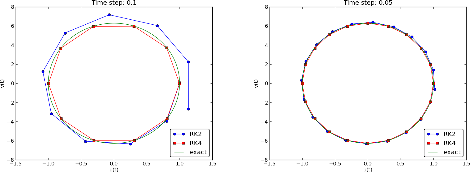
Phase plane plot of the numerical solutions
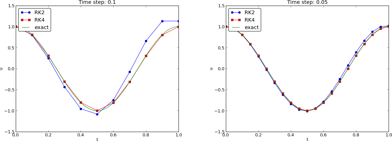
Plain solution curves
Observations from the figures
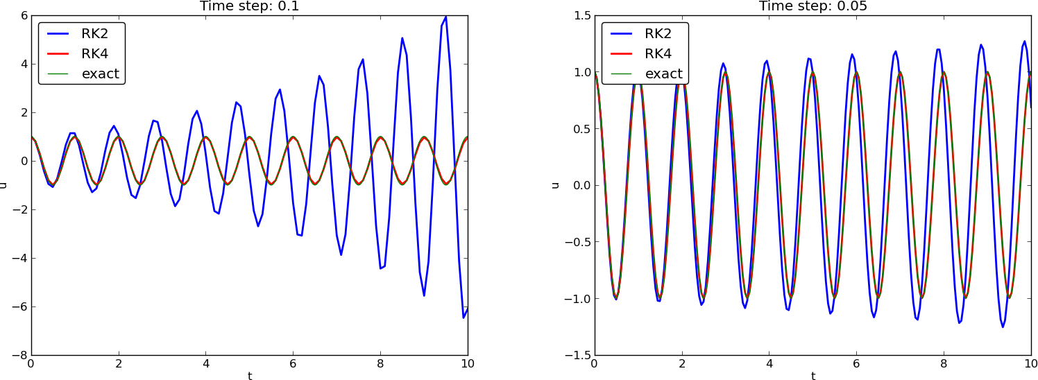
Runge-Kutta methods of order 2 and 4; short time series
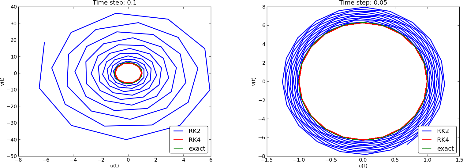
Runge-Kutta methods of order 2 and 4; longer time series
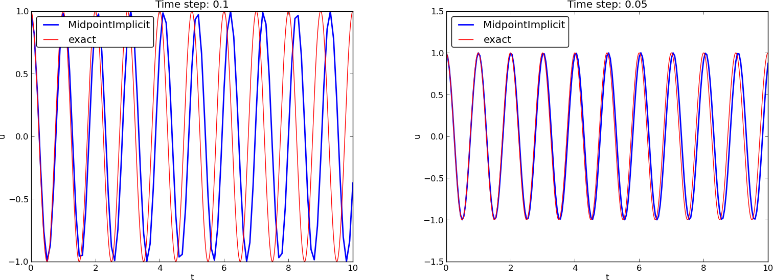
Crank-Nicolson; longer time series
Observations of RK and CN methods
Energy conservation property
Derivation of the energy conservation property
Remark about \( E(t) \)
The Euler-Cromer method; idea
The Euler-Cromer method; complete formulas
Euler-Cromer is equivalent to the scheme for \( u^{\prime\prime}+\omega^2u=0 \)
The schemes are not equivalent wrt the initial conditions
Generalization: damping, nonlinear spring, and external excitation
A centered scheme for linear damping
Initial conditions
Linearization via a geometric mean approximation
A centered scheme for quadratic damping
Initial condition for quadratic damping
Algorithm
Implementation
Verification
Demo program
Euler-Cromer formulation
Staggered grid
Linear damping
Quadratic damping
Initial conditions
Exact solution: $$ u(t) = I\cos (\omega t) $$ \( u(t) \) oscillates with constant amplitude \( I \) and (angular) frequency \( \omega \). Period: \( P=2\pi/\omega \).
Step 3: Approximate derivative(s) by finite difference approximation(s). Very common (standard!) formula for \( u^{\prime\prime} \): $$ u^{\prime\prime}(t_n) \approx \frac{u^{n+1}-2u^n + u^{n-1}}{\Delta t^2} $$
Use this discrete initial condition together with the ODE at \( t=0 \) to eliminate \( u^{-1} \): $$ \frac{u^{n+1}-2u^n + u^{n-1}}{\Delta t^2} = -\omega^2 u^n $$
Step 4: Formulate the computational algorithm. Assume \( u^{n-1} \) and \( u^n \) are known, solve for unknown \( u^{n+1} \): $$ u^{n+1} = 2u^n - u^{n-1} - \Delta t^2\omega^2 u^n $$
Nick names for this scheme: Stormer's method or Verlet integration.
Inserted in the scheme for \( n=0 \) gives $$ u^1 = u^0 - \half \Delta t^2 \omega^2 u^0 $$
t = linspace(0, T, Nt+1)  # mesh points in time
dt = t[1] - t[0]          # constant time step.
u = zeros(Nt+1)           # solution

u[0] = I
u[1] = u[0] - 0.5*dt**2*w**2*u[0]
for n in range(1, Nt):
    u[n+1] = 2*u[n] - u[n-1] - dt**2*w**2*u[n]
Note: w is consistently used for \( \omega \) in my code.
With \( [D_tD_t u]^n \) as the finite difference approximation to \( u^{\prime\prime}(t_n) \) we can write $$ [D_tD_t u + \omega^2 u = 0]^n $$
\( [D_tD_t u]^n \) means applying a central difference with step \( \Delta t/2 \) twice: $$ [D_t(D_t u)]^n = \frac{[D_t u]^{n+\half} - [D_t u]^{n-\half}}{\Delta t}$$ which is written out as $$ \frac{1}{\Delta t}\left(\frac{u^{n+1}-u^n}{\Delta t} - \frac{u^{n}-u^{n-1}}{\Delta t}\right) = \frac{u^{n+1}-2u^n + u^{n-1}}{\Delta t^2} \tp $$
\( u \) is often displacement/position, \( u^{\prime} \) is velocity and can be computed by $$ u^{\prime}(t_n) \approx \frac{u^{n+1}-u^{n-1}}{2\Delta t} = [D_{2t}u]^n $$
import numpy as np
import matplotlib.pyplot as plt

def solver(I, w, dt, T):
    """
    Solve u'' + w**2*u = 0 for t in (0,T], u(0)=I and u'(0)=0,
    by a central finite difference method with time step dt.
    """
    dt = float(dt)
    Nt = int(round(T/dt))
    u = np.zeros(Nt+1)
    t = np.linspace(0, Nt*dt, Nt+1)

    u[0] = I
    u[1] = u[0] - 0.5*dt**2*w**2*u[0]
    for n in range(1, Nt):
        u[n+1] = 2*u[n] - u[n-1] - dt**2*w**2*u[n]
    return u, t
def u_exact(t, I, w):
    return I*np.cos(w*t)

def visualize(u, t, I, w):
    plt.plot(t, u, 'r--o')
    t_fine = np.linspace(0, t[-1], 1001)  # very fine mesh for u_e
    u_e = u_exact(t_fine, I, w)
    plt.hold('on')
    plt.plot(t_fine, u_e, 'b-')
    plt.legend(['numerical', 'exact'], loc='upper left')
    plt.xlabel('t')
    plt.ylabel('u')
    dt = t[1] - t[0]
    plt.title('dt=%g' % dt)
    umin = 1.2*u.min();  umax = -umin
    plt.axis([t[0], t[-1], umin, umax])
    plt.savefig('tmp1.png');  plt.savefig('tmp1.pdf')
I = 1
w = 2*pi
dt = 0.05
num_periods = 5
P = 2*pi/w    #  one period
T = P*num_periods
u, t = solver(I, w, dt, T)
visualize(u, t, I, w, dt)
import argparse
parser = argparse.ArgumentParser()
parser.add_argument('--I', type=float, default=1.0)
parser.add_argument('--w', type=float, default=2*pi)
parser.add_argument('--dt', type=float, default=0.05)
parser.add_argument('--num_periods', type=int, default=5)
a = parser.parse_args()
I, w, dt, num_periods = a.I, a.w, a.dt, a.num_periods
Terminal> python vib_undamped.py --dt 0.05 --num_periods 40
Generates frames tmp_vib%04d.png in files. Can make movie:
Terminal> ffmpeg -r 12 -i tmp_vib%04d.png -c:v flv movie.flv
Can use avconv instead of ffmpeg.
| Format | Codec and filename |
|---|---|
| Flash | -c:v flv movie.flv |
| MP4 | -c:v libx264 movie.mp4 |
| Webm | -c:v libvpx movie.webm |
| Ogg | -c:v libtheora movie.ogg |
The next function estimates convergence rates, i.e., it
def convergence_rates(m, solver_function, num_periods=8):
    """
    Return m-1 empirical estimates of the convergence rate
    based on m simulations, where the time step is halved
    for each simulation.
    solver_function(I, w, dt, T) solves each problem, where T
    is based on simulation for num_periods periods.
    """
    from math import pi
    w = 0.35; I = 0.3       # just chosen values
    P = 2*pi/w              # period
    dt = P/30               # 30 time step per period 2*pi/w
    T = P*num_periods

    dt_values = []
    E_values = []
    for i in range(m):
        u, t = solver_function(I, w, dt, T)
        u_e = u_exact(t, I, w)
        E = np.sqrt(dt*np.sum((u_e-u)**2))
        dt_values.append(dt)
        E_values.append(E)
        dt = dt/2

    r = [np.log(E_values[i-1]/E_values[i])/
         np.log(dt_values[i-1]/dt_values[i])
         for i in range(1, m, 1)]
    return r
Result: r contains values equal to 2.00 - as expected!
Use final r[-1] in a unit test:
def test_convergence_rates():
    r = convergence_rates(m=5, solver_function=solver, num_periods=8)
    # Accept rate to 1 decimal place
    tol = 0.1
    assert abs(r[-1] - 2.0) < tol
Complete code in vib_undamped.py.
scitools.MovingPlotWindow.scitools.avplotter (ASCII vertical plotter).
Terminal> python vib_undamped.py --dt 0.05 --num_periods 40
Movie of the moving plot window.
!splot
!splot
def bokeh_plot(u, t, legends, I, w, t_range, filename):
    """
    Make plots for u vs t using the Bokeh library.
    u and t are lists (several experiments can be compared).
    legens contain legend strings for the various u,t pairs.
    """
    if not isinstance(u, (list,tuple)):
        u = [u]  # wrap in list
    if not isinstance(t, (list,tuple)):
        t = [t]  # wrap in list
    if not isinstance(legends, (list,tuple)):
        legends = [legends]  # wrap in list

    import bokeh.plotting as plt
    plt.output_file(filename, mode='cdn', title='Comparison')
    # Assume that all t arrays have the same range
    t_fine = np.linspace(0, t[0][-1], 1001)  # fine mesh for u_e
    tools = 'pan,wheel_zoom,box_zoom,reset,'\
            'save,box_select,lasso_select'
    u_range = [-1.2*I, 1.2*I]
    font_size = '8pt'
    p = []  # list of plot objects
    # Make the first figure
    p_ = plt.figure(
        width=300, plot_height=250, title=legends[0],
        x_axis_label='t', y_axis_label='u',
        x_range=t_range, y_range=u_range, tools=tools,
        title_text_font_size=font_size)
    p_.xaxis.axis_label_text_font_size=font_size
    p_.yaxis.axis_label_text_font_size=font_size
    p_.line(t[0], u[0], line_color='blue')
    # Add exact solution
    u_e = u_exact(t_fine, I, w)
    p_.line(t_fine, u_e, line_color='red', line_dash='4 4')
    p.append(p_)
    # Make the rest of the figures and attach their axes to
    # the first figure's axes
    for i in range(1, len(t)):
        p_ = plt.figure(
            width=300, plot_height=250, title=legends[i],
            x_axis_label='t', y_axis_label='u',
            x_range=p[0].x_range, y_range=p[0].y_range, tools=tools,
            title_text_font_size=font_size)
        p_.xaxis.axis_label_text_font_size = font_size
        p_.yaxis.axis_label_text_font_size = font_size
        p_.line(t[i], u[i], line_color='blue')
        p_.line(t_fine, u_e, line_color='red', line_dash='4 4')
        p.append(p_)

    # Arrange all plots in a grid with 3 plots per row
    grid = [[]]
    for i, p_ in enumerate(p):
        grid[-1].append(p_)
        if (i+1) % 3 == 0:
            # New row
            grid.append([])
    plot = plt.gridplot(grid, toolbar_location='left')
    plt.save(plot)
    plt.show(plot)
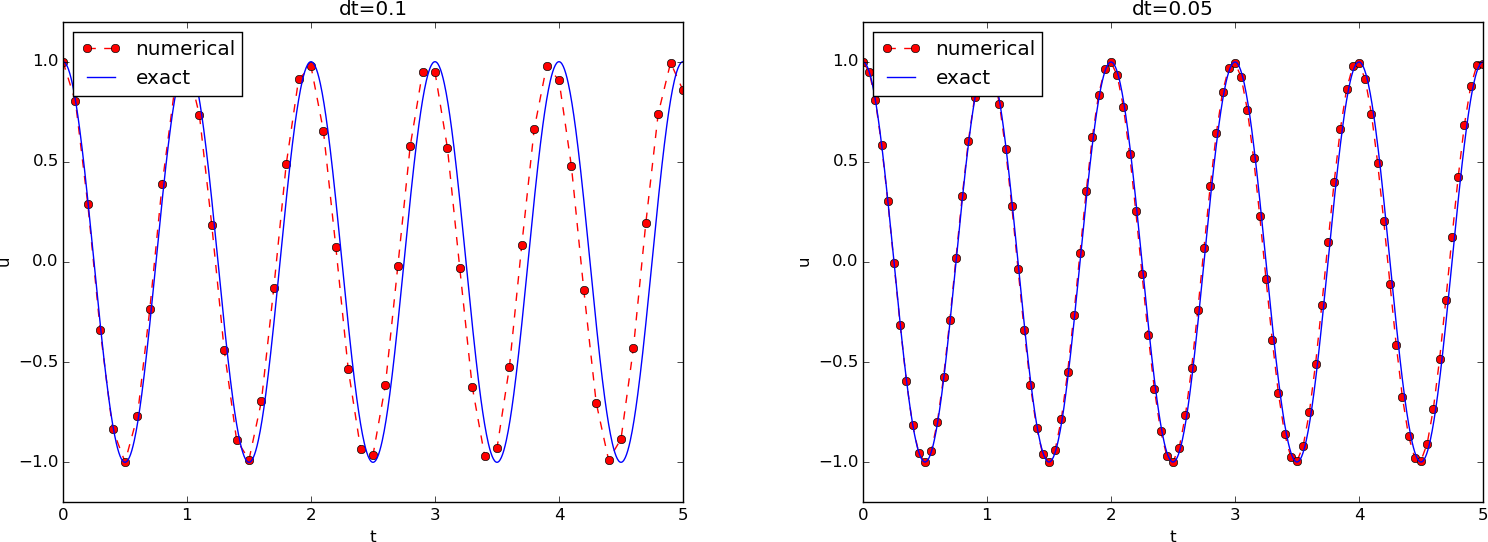
\( u^{\prime\prime} + \omega^2 u = 0 \), \( u(0)=1 \), \( u^{\prime}(0)=0 \),
\( \omega=2\pi \), \( \uex(t)=\cos (2\pi t) \), \( \Delta t = 0.05 \) (20 intervals
per period)
The scheme with \( u^n=I\exp{(i\omega\tilde\Delta t\, n)} \) inserted gives $$ -I\exp{(i\tilde\omega t)}\frac{4}{\Delta t^2}\sin^2(\frac{\tilde\omega\Delta t}{2}) + \omega^2 I\exp{(i\tilde\omega t)} = 0 $$ which after dividing by \( I\exp{(i\tilde\omega t)} \) results in $$ \frac{4}{\Delta t^2}\sin^2(\frac{\tilde\omega\Delta t}{2}) = \omega^2 $$ Solve for \( \tilde\omega \): $$ \tilde\omega = \pm \frac{2}{\Delta t}\sin^{-1}\left(\frac{\omega\Delta t}{2}\right) $$
Taylor series expansion for small \( \Delta t \) gives a formula that is easier to understand:
>>> from sympy import *
>>> dt, w = symbols('dt w')
>>> w_tilde = asin(w*dt/2).series(dt, 0, 4)*2/dt
>>> print w_tilde
(dt*w + dt**3*w**3/24 + O(dt**4))/dt  # note the final "/dt"
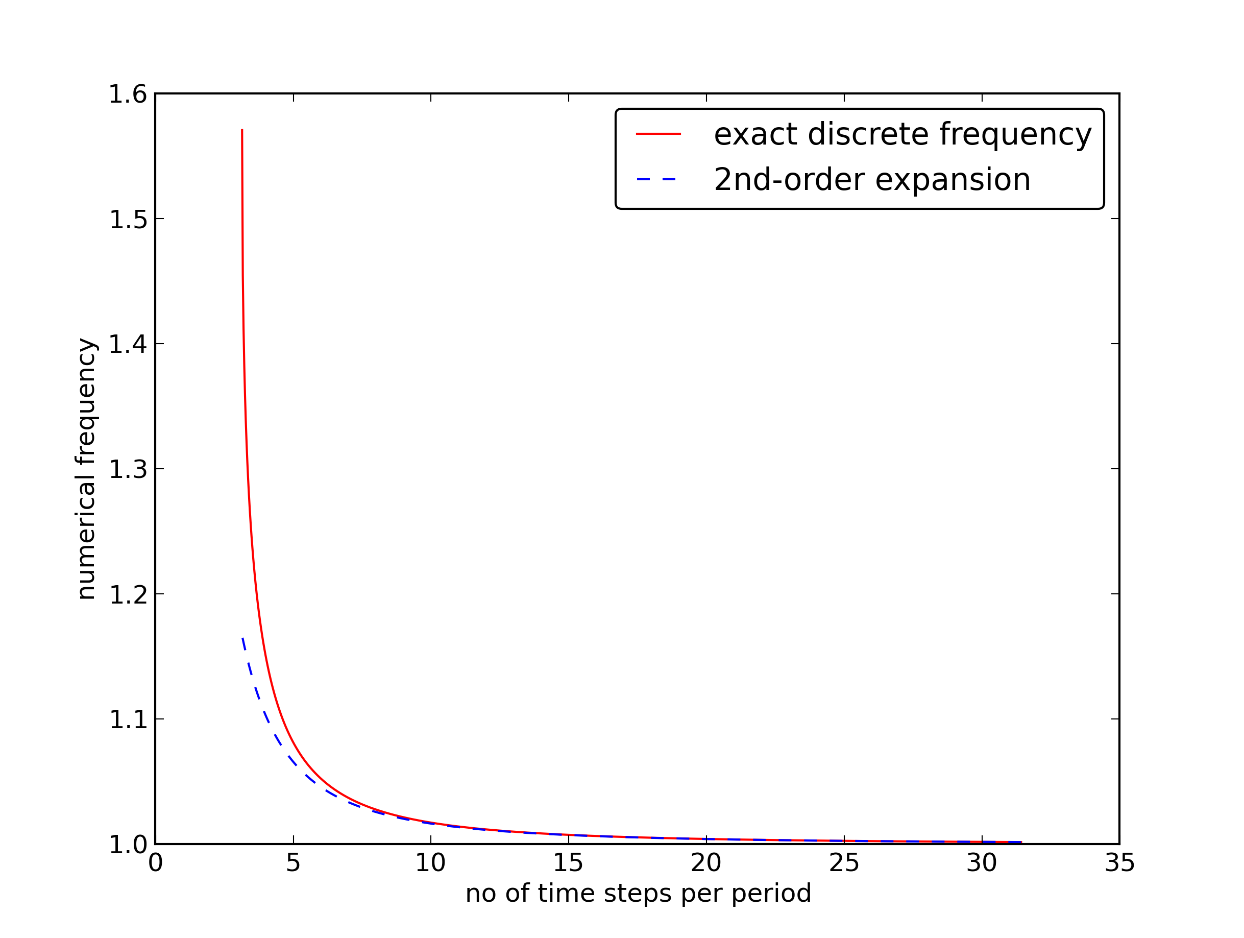
Recommendation: 25-30 points per period.
The error mesh function, $$ e^n = \uex(t_n) - u^n = I\cos\left(\omega n\Delta t\right) - I\cos\left(\tilde\omega n\Delta t\right) $$ is ideal for verification and further analysis! $$ e^n = I\cos\left(\omega n\Delta t\right) - I\cos\left(\tilde\omega n\Delta t\right) = -2I\sin\left(t\half\left( \omega - \tilde\omega\right)\right) \sin\left(t\half\left( \omega + \tilde\omega\right)\right) $$
Can easily show convergence:
$$ e^n\rightarrow 0 \hbox{ as }\Delta t\rightarrow 0,$$
because
$$
\lim_{\Delta t\rightarrow 0}
\tilde\omega = \lim_{\Delta t\rightarrow 0}
\frac{2}{\Delta t}\sin^{-1}\left(\frac{\omega\Delta t}{2}\right)
= \omega,
$$
by L'Hopital's rule or simply asking sympy:
or WolframAlpha:
>>> import sympy as sym
>>> dt, w = sym.symbols('x w')
>>> sym.limit((2/dt)*sym.asin(w*dt/2), dt, 0, dir='+')
w
Observations:
Cannot tolerate growth and must therefore demand a stability criterion $$ \frac{\omega\Delta t}{2} \leq 1\quad\Rightarrow\quad \Delta t \leq \frac{2}{\omega} $$
Try \( \Delta t = \frac{2}{\omega} + 9.01\cdot 10^{-5} \) (slightly too big!):
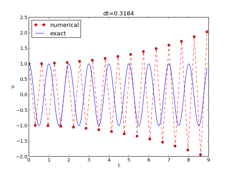
We can draw three important conclusions:
The vast collection of ODE solvers (e.g., in Odespy) cannot be applied to $$ u^{\prime\prime} + \omega^2 u = 0$$ unless we write this higher-order ODE as a system of 1st-order ODEs.
Introduce an auxiliary variable \( v=u^{\prime} \): $$ \begin{align} u^{\prime} &= v, \label{vib:model2x2:ueq}\\ v^{\prime} &= -\omega^2 u \label{vib:model2x2:veq} \tp \end{align} $$
Initial conditions: \( u(0)=I \) and \( v(0)=0 \).
We apply the Forward Euler scheme to each component equation: $$ [D_t^+ u = v]^n,$$ $$ [D_t^+ v = -\omega^2 u]^n,$$ or written out, $$ \begin{align} u^{n+1} &= u^n + \Delta t v^n, \label{_auto1}\\ v^{n+1} &= v^n -\Delta t \omega^2 u^n \tp \label{_auto2} \end{align} $$
We apply the Backward Euler scheme to each component equation: $$ [D_t^- u = v]^{n+1},$$ $$ [D_t^- v = -\omega u]^{n+1} \tp $$ Written out: $$ \begin{align} u^{n+1} - \Delta t v^{n+1} = u^{n}, \label{_auto3}\\ v^{n+1} + \Delta t \omega^2 u^{n+1} = v^{n} \tp \label{_auto4} \end{align} $$ This is a coupled \( 2\times 2 \) system for the new values at \( t=t_{n+1} \)!
Can use Odespy to compare many methods for first-order schemes:
import odespy
import numpy as np

def f(u, t, w=1):
    u, v = u  # u is array of length 2 holding our [u, v]
    return [v, -w**2*u]

def run_solvers_and_plot(solvers, timesteps_per_period=20,
                         num_periods=1, I=1, w=2*np.pi):
    P = 2*np.pi/w  # duration of one period
    dt = P/timesteps_per_period
    Nt = num_periods*timesteps_per_period
    T = Nt*dt
    t_mesh = np.linspace(0, T, Nt+1)

    legends = []
    for solver in solvers:
        solver.set(f_kwargs={'w': w})
        solver.set_initial_condition([I, 0])
        u, t = solver.solve(t_mesh)
solvers = [
    odespy.ForwardEuler(f),
    # Implicit methods must use Newton solver to converge
    odespy.BackwardEuler(f, nonlinear_solver='Newton'),
    odespy.CrankNicolson(f, nonlinear_solver='Newton'),
    ]
Two plot types:
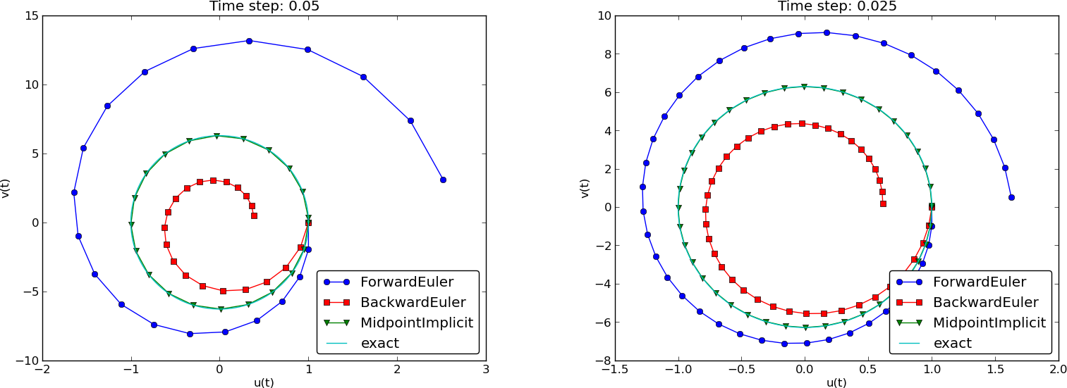
Note: CrankNicolson in Odespy leads to the name MidpointImplicit in plots.
Figure 1: Comparison of classical schemes.
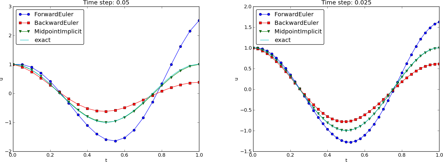
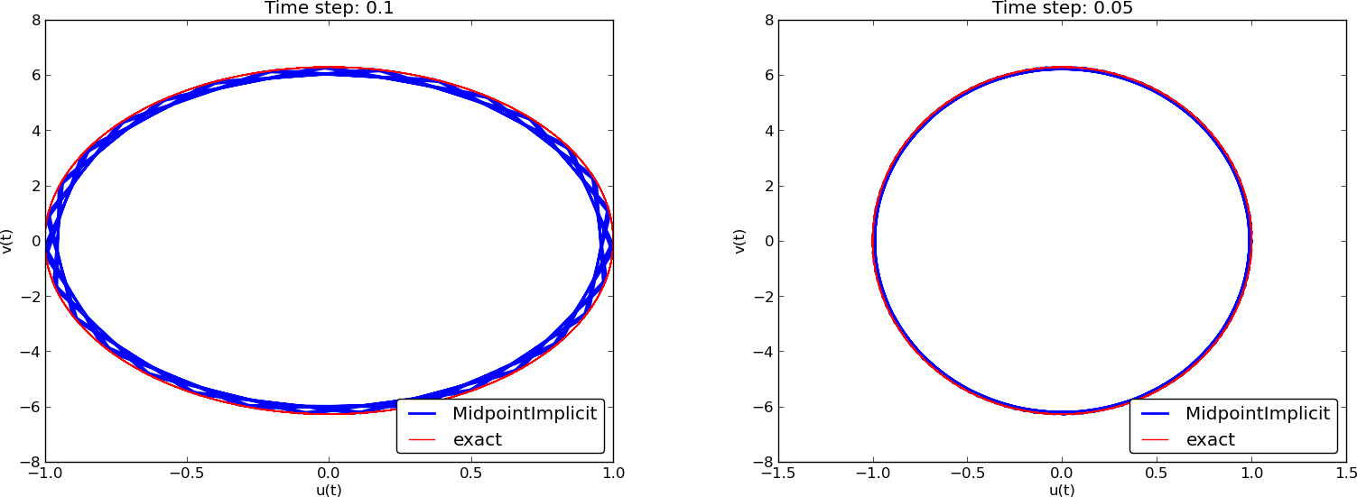
(MidpointImplicit means CrankNicolson in Odespy)
The model $$ u^{\prime\prime} + \omega^2 u = 0,\quad u(0)=I,\ u^{\prime}(0)=V,$$ has the nice energy conservation property that $$ E(t) = \half(u^{\prime})^2 + \half\omega^2u^2 = \hbox{const}\tp$$ This can be used to check solutions.
Multiply \( u^{\prime\prime}+\omega^2u=0 \) by \( u^{\prime} \) and integrate: $$ \int_0^T u^{\prime\prime}u^{\prime} dt + \int_0^T\omega^2 u u^{\prime} dt = 0\tp$$ Observing that $$ u^{\prime\prime}u^{\prime} = \frac{d}{dt}\half(u^{\prime})^2,\quad uu^{\prime} = \frac{d}{dt} {\half}u^2,$$ we get $$ \int_0^T (\frac{d}{dt}\half(u^{\prime})^2 + \frac{d}{dt} \half\omega^2u^2)dt = E(T) - E(0), $$ where $$ E(t) = \half(u^{\prime})^2 + \half\omega^2u^2 $$
\( E(t) \) does not measure energy, energy per mass unit.
Starting with an ODE coming directly from Newton's 2nd law \( F=ma \) with a spring force \( F=-ku \) and \( ma=mu^{\prime\prime} \) (\( a \): acceleration, \( u \): displacement), we have $$ mu^{\prime\prime} + ku = 0$$ Integrating this equation gives a physical energy balance: $$ E(t) = \underbrace{{\half}mv^2}_{\hbox{kinetic energy} } + \underbrace{{\half}ku^2}_{\hbox{potential energy}} = E(0),\quad v=u^{\prime} $$ Note: the balance is not valid if we add other terms to the ODE.
2x2 system for \( u^{\prime\prime}+\omega^2u=0 \): $$ \begin{align*} v^{\prime} &= -\omega^2u\\ u^{\prime} &= v \end{align*} $$
Forward-backward discretization:
Written out: $$ \begin{align} u^0 &= I, \label{_auto9}\\ v^0 &= 0, \label{_auto10}\\ v^{n+1} &= v^n -\Delta t \omega^2u^{n} \label{vib:model2x2:EulerCromer:veq1}\\ u^{n+1} &= u^n + \Delta t v^{n+1} \label{vib:model2x2:EulerCromer:ueq1} \end{align} $$
Names: Forward-backward scheme, Semi-implicit Euler method, symplectic Euler, semi-explicit Euler, Newton-Stormer-Verlet, and Euler-Cromer.
which is the centered finite differrence scheme for \( u^{\prime\prime}+\omega^2u=0 \)!
The exact discrete solution derived earlier does not fit the Euler-Cromer scheme because of mismatch for \( u^1 \).
Typical choices of \( f \) and \( s \):
\( u(0)=I \), \( u'(0)=V \): $$ \begin{align*} \lbrack u &=I\rbrack^0\quad\Rightarrow\quad u^0=I\\ \lbrack D_{2t}u &=V\rbrack^0\quad\Rightarrow\quad u^{-1} = u^{1} - 2\Delta t V \end{align*} $$ End result: $$ u^1 = u^0 + \Delta t\, V + \frac{\Delta t^2}{2m}(-bV - s(u^0) + F^0) $$ Same formula for \( u^1 \) as when using a centered scheme for \( u''+\omega u=0 \).
After some algebra: $$ \begin{align*} u^{n+1} &= \left( m + b|u^n-u^{n-1}|\right)^{-1}\times \\ & \qquad \left(2m u^n - mu^{n-1} + bu^n|u^n-u^{n-1}| + \Delta t^2 (F^n - s(u^n)) \right) \end{align*} $$
Simply use that \( u'=V \) in the scheme when \( t=0 \) (\( n=0 \)): $$ [mD_tD_t u + bV|V| + s(u) = F]^0 $$
which gives $$ u^1 = u^0 + \Delta t V + \frac{\Delta t^2}{2m}\left(-bV|V| - s(u^0) + F^0\right) $$
def solver(I, V, m, b, s, F, dt, T, damping='linear'):
    dt = float(dt); b = float(b); m = float(m) # avoid integer div.
    Nt = int(round(T/dt))
    u = zeros(Nt+1)
    t = linspace(0, Nt*dt, Nt+1)

    u[0] = I
    if damping == 'linear':
        u[1] = u[0] + dt*V + dt**2/(2*m)*(-b*V - s(u[0]) + F(t[0]))
    elif damping == 'quadratic':
        u[1] = u[0] + dt*V + \
               dt**2/(2*m)*(-b*V*abs(V) - s(u[0]) + F(t[0]))

    for n in range(1, Nt):
        if damping == 'linear':
            u[n+1] = (2*m*u[n] + (b*dt/2 - m)*u[n-1] +
                      dt**2*(F(t[n]) - s(u[n])))/(m + b*dt/2)
        elif damping == 'quadratic':
            u[n+1] = (2*m*u[n] - m*u[n-1] + b*u[n]*abs(u[n] - u[n-1])
                      + dt**2*(F(t[n]) - s(u[n])))/\
                      (m + b*abs(u[n] - u[n-1]))
    return u, t
vib.py supports input via the command line:
Terminal> python vib.py --s 'sin(u)' --F '3*cos(4*t)' --c 0.03
This results in a moving window following the function on the screen.
We rewrite $$ mu'' + f(u') + s(u) = F(t),\quad u(0)=I,\ u'(0)=V,\ t\in (0,T] $$ as a first-order ODE system $$ \begin{align*} u' &= v \\ v' &= m^{-1}\left(F(t) - f(v) - s(u)\right) \end{align*} $$
Written out, $$ \begin{align*} \frac{u^n - u^{n-1}}{\Delta t} &= v^{n-\half}\\ \frac{v^{n+\half} - v^{n-\half}}{\Delta t} &= m^{-1}\left(F^n - f(v^n) - s(u^n)\right) \end{align*} $$
Problem: \( f(v^n) \)
With \( f(v)=bv \), we can use an arithmetic mean for \( bv^n \) a la Crank-Nicolson schemes. $$ \begin{align*} u^n & = u^{n-1} + {\Delta t}v^{n-\half},\\ v^{n+\half} &= \left(1 + \frac{b}{2m}\Delta t\right)^{-1}\left( v^{n-\half} + {\Delta t} m^{-1}\left(F^n - {\half}f(v^{n-\half}) - s(u^n)\right)\right)\tp \end{align*} $$
With \( f(v)=b|v|v \), we can use a geometric mean $$ b|v^n|v^n\approx b|v^{n-\half}|v^{n+\half}, $$ resulting in $$ \begin{align*} u^n & = u^{n-1} + {\Delta t}v^{n-\half},\\ v^{n+\half} &= (1 + \frac{b}{m}|v^{n-\half}|\Delta t)^{-1}\left( v^{n-\half} + {\Delta t} m^{-1}\left(F^n - s(u^n)\right)\right)\tp \end{align*} $$