$$ \newcommand{\half}{\frac{1}{2}} \newcommand{\tp}{\thinspace .} \newcommand{\uex}{{u_{\small\mbox{e}}}} \newcommand{\x}{\boldsymbol{x}} \newcommand{\X}{\boldsymbol{X}} \renewcommand{\v}{\boldsymbol{v}} \newcommand{\dfc}{\alpha} % diffusion coefficient \newcommand{\If}{\mathcal{I}_s} % for FEM \newcommand{\Ifb}{{I_b}} % for FEM \newcommand{\sequencei}[1]{\left\{ {#1}_i \right\}_{i\in\If}} \newcommand{\basphi}{\varphi} \newcommand{\baspsi}{\psi} \newcommand{\refphi}{\tilde\basphi} \newcommand{\sinL}[1]{\sin\left((#1+1)\pi\frac{x}{L}\right)} \newcommand{\xno}[1]{x_{#1}} \newcommand{\dX}{\, \mathrm{d}X} \newcommand{\dx}{\, \mathrm{d}x} \newcommand{\ds}{\, \mathrm{d}s} $$

Study guide: Computing with variational forms

Hans Petter Langtangen [1, 2]

[1] Center for Biomedical Computing, Simula Research Laboratory [2] Department of Informatics, University of Oslo

2016

Basic principles for approximating differential equations

We shall apply least squares, Galerkin/projection, and collocation to differential equation models

Our aim is to extend the ideas for approximating $ f $ by $ u $, or solving $$ u = f $$

to real, spatial differential equations like $$ -u'' + bu = f,\quad u(0)=C,\ u'(L)=D $$

Emphasis will be on the Galerkin/projection method

Abstract differential equation

$$ \begin{equation*} \mathcal{L}(u) = 0,\quad x\in\Omega \end{equation*} $$

Examples (1D problems): $$ \begin{align*} \mathcal{L}(u) &= \frac{d^2u}{dx^2} - f(x),\\ \mathcal{L}(u) &= \frac{d}{dx}\left(\dfc(x)\frac{du}{dx}\right) + f(x),\\ \mathcal{L}(u) &= \frac{d}{dx}\left(\dfc(u)\frac{du}{dx}\right) - au + f(x),\\ \mathcal{L}(u) &= \frac{d}{dx}\left(\dfc(u)\frac{du}{dx}\right) + f(u,x) \end{align*} $$

Abstract boundary conditions

$$ \begin{equation*} \mathcal{B}_0(u)=0,\ x=0,\quad \mathcal{B}_1(u)=0,\ x=L \end{equation*} $$

Examples: $$ \begin{align*} \mathcal{B}_i(u) &= u - g,\quad &\hbox{Dirichlet condition}\\ \mathcal{B}_i(u) &= -\dfc \frac{du}{dx} - g,\quad &\hbox{Neumann condition}\\ \mathcal{B}_i(u) &= -\dfc \frac{du}{dx} - h(u-g),\quad &\hbox{Robin condition} \end{align*} $$

Reminder about notation

$ \uex(x) $ is the symbol for the exact solution of $ \mathcal{L}(\uex)=0 $ and $ \mathcal{B}_i (\uex)=0 $

$ u(x) $ denotes an approximate solution

$ V = \hbox{span}\{ \baspsi_0(x),\ldots,\baspsi_N(x)\} $, $ V $ has basis $ \sequencei{\baspsi} $

We seek $ u\in V $

$ \If =\{0,\ldots,N\} $ is an index set

$ u(x) = \sum_{j\in\If} c_j\baspsi_j(x) $

Inner product: $ (u,v) = \int_\Omega uv\dx $

Norm: $ ||u||=\sqrt{(u,u)} $

New topics: variational formulation and boundary conditions

Much is similar to approximating a function (solving $ u=f $), but two new topics are needed:

Variational formulation of the differential equation problem (including integration by parts)

Handling of boundary conditions

Residual-minimizing principles

When solving $ u=f $ we knew the error $ e=f-u $ and could use principles for minimizing the error

When solving $ \mathcal{L}(\uex)=0 $ we do not know $ \uex $ and cannot work with the error $ e=\uex - u $

We can only know the error in the equation: the residual $ R $

Inserting $ u=\sum_jc_j\baspsi_j $ in $ \mathcal{L}=0 $ gives a residual $ R $ $$ \begin{equation*} \mathcal{L}(u) = \mathcal{L}(\sum_j c_j \baspsi_j) = R \neq 0 \end{equation*} $$

Goal: minimize $ R $ with respect to $ \sequencei{c} $ (and hope it makes a small $ e $ too) $$ R=R(c_0,\ldots,c_N; x)$$

The least squares method

Idea: minimize $$ \begin{equation*} E = ||R||^2 = (R,R) = \int_{\Omega} R^2 dx \end{equation*} $$

Minimization wrt $ \sequencei{c} $ implies $$ \frac{\partial E}{\partial c_i} = \int_{\Omega} 2R\frac{\partial R}{\partial c_i} dx = 0\quad \Leftrightarrow\quad (R,\frac{\partial R}{\partial c_i})=0,\quad i\in\If $$

$ N+1 $ equations for $ N+1 $ unknowns $ \sequencei{c} $

The Galerkin method

Idea: make $ R $ orthogonal to $ V $, $$ (R,v)=0,\quad \forall v\in V $$

This implies $$ (R,\baspsi_i)=0,\quad i\in\If $$

$ N+1 $ equations for $ N+1 $ unknowns $ \sequencei{c} $

The Method of Weighted Residuals

Generalization of the Galerkin method: demand $ R $ orthogonal to some space $ W $, possibly $ W\neq V $: $$ (R,v)=0,\quad \forall v\in W $$

If $ \{w_0,\ldots,w_N\} $ is a basis for $ W $: $$ (R,w_i)=0,\quad i\in\If $$

$ N+1 $ equations for $ N+1 $ unknowns $ \sequencei{c} $

Weighted residual with $ w_i = \partial R/\partial c_i $ gives least squares

New terminology: test and trial functions

$ \baspsi_j $ used in $ \sum_jc_j\baspsi_j $ is called trial function

$ \baspsi_i $ or $ w_i $ used as weight in Galerkin's method is called test function

The collocation method

Idea: demand $ R=0 $ at $ N+1 $ points in space $$ R(\xno{i}; c_0,\ldots,c_N)=0,\quad i\in\If$$

The collocation method is a weighted residual method with delta functions as weights $$ 0 = \int_\Omega R(x;c_0,\ldots,c_N) \delta(x-\xno{i})\dx = R(\xno{i}; c_0,\ldots,c_N)$$ $$ \hbox{property of } \delta(x):\quad \int_{\Omega} f(x)\delta (x-\xno{i}) dx = f(\xno{i}),\quad \xno{i}\in\Omega $$

Examples on using the principles

Goal.

Exemplify the least squares, Galerkin, and collocation methods in a simple 1D problem with global basis functions.

The first model problem

$$ -u''(x) = f(x),\quad x\in\Omega=[0,L],\quad u(0)=0,\ u(L)=0$$

Basis functions: $$ \baspsi_i(x) = \sinL{i},\quad i\in\If$$

Residual: $$ \begin{align*} R(x;c_0,\ldots,c_N) &= u''(x) + f(x),\nonumber\\ &= \frac{d^2}{dx^2}\left(\sum_{j\in\If} c_j\baspsi_j(x)\right) + f(x),\nonumber\\ &= \sum_{j\in\If} c_j\baspsi_j''(x) + f(x) \end{align*} $$

Boundary conditions

Since $ u(0)=u(L)=0 $ we must ensure that all $ \baspsi_i(0)=\baspsi_i(L)=0 $, because then $$ u(0) = \sum_jc_j{\color{red}\baspsi_j(0)} = 0,\quad u(L) = \sum_jc_j{\color{red}\baspsi_j(L)} =0 $$

$ u $ known: Dirichlet boundary condition

$ u' $ known: Neumann boundary condition

Must have $ \baspsi_i=0 $ where Dirichlet conditions apply

The least squares method; principle

$$ (R,\frac{\partial R}{\partial c_i}) = 0,\quad i\in\If $$ $$ \begin{equation*} \frac{\partial R}{\partial c_i} = \frac{\partial}{\partial c_i} \left(\sum_{j\in\If} c_j\baspsi_j''(x) + f(x)\right) = \baspsi_i''(x) \end{equation*} $$

Because: $$ \frac{\partial}{\partial c_i}\left(c_0\baspsi_0'' + c_1\baspsi_1'' + \cdots + c_{i-1}\baspsi_{i-1}'' + {\color{red}c_i\baspsi_{i}''} + c_{i+1}\baspsi_{i+1}'' + \cdots + c_N\baspsi_N'' \right) = \baspsi_{i}'' $$

The least squares method; equation system

$$ \begin{equation*} (\sum_j c_j \baspsi_j'' + f,\baspsi_i'')=0,\quad i\in\If \end{equation*} $$

Rearrangement: $$ \begin{equation*} \sum_{j\in\If}(\baspsi_i'',\baspsi_j'')c_j = -(f,\baspsi_i''),\quad i\in\If \end{equation*} $$

This is a linear system $$ \begin{equation*} \sum_{j\in\If}A_{i,j}c_j = b_i,\quad i\in\If \end{equation*} $$

The least squares method; matrix and right-hand side expressions

$$ \begin{align*} A_{i,j} &= (\baspsi_i'',\baspsi_j'')\nonumber\\ & = \pi^4(i+1)^2(j+1)^2L^{-4}\int_0^L \sinL{i}\sinL{j}\, dx\nonumber\\ &= \left\lbrace \begin{array}{ll} {1\over2}L^{-3}\pi^4(i+1)^4 & i=j \\ 0, & i\neq j \end{array}\right. \\ b_i &= -(f,\baspsi_i'') = (i+1)^2\pi^2L^{-2}\int_0^Lf(x)\sinL{i}\, dx \end{align*} $$

Orthogonality of the basis functions gives diagonal matrix

Useful property of the chosen basis functions: $$ \begin{equation*} \int\limits_0^L \sinL{i}\sinL{j}\, dx = \delta_{ij},\quad \quad\delta_{ij} = \left\lbrace \begin{array}{ll} \half L & i=j \\ 0, & i\neq j \end{array}\right. \end{equation*} $$

$ \Rightarrow\ (\baspsi_i'',\baspsi_j'') = \delta_{ij} $, i.e., diagonal $ A_{i,j} $, and we can easily solve for $ c_i $: $$ \begin{equation*} c_i = \frac{2L}{\pi^2(i+1)^2}\int_0^Lf(x)\sinL{i}\, dx \end{equation*} $$

Least squares method; solution

Let sympy do the work ($ f(x)=2 $):

1 2 3 4 5 6 7 8 9 10
from sympy import * import sys i, j = symbols('i j', integer=True) x, L = symbols('x L') f = 2 a = 2*L/(pi**2*(i+1)**2) c_i = a*integrate(f*sin((i+1)*pi*x/L), (x, 0, L)) c_i = simplify(c_i) print c_i

$$ \begin{equation*} c_i = 4 \frac{L^{2} \left(\left(-1\right)^{i} + 1\right)}{\pi^{3} \left(i^{3} + 3 i^{2} + 3 i + 1\right)},\quad u(x) = \sum_{k=0}^{N/2} \frac{8L^2}{\pi^3(2k+1)^3}\sinL{2k} \end{equation*} $$

Fast decay: $ c_2 = c_0/27 $, $ c_4=c_0/125 $ - only one term might be good enough: $$ \begin{equation*} u(x) \approx \frac{8L^2}{\pi^3}\sin\left(\pi\frac{x}{L}\right) \end{equation*} $$

The Galerkin method; principle

$ R=u''+f $: $$ \begin{equation*} (u''+f,v)=0,\quad \forall v\in V, \end{equation*} $$ or rearranged, $$ \begin{equation*} (u'',v) = -(f,v),\quad\forall v\in V \end{equation*} $$

This is a variational formulation of the differential equation problem.

$ \forall v\in V $ is equivalent with $ \forall v\in\baspsi_i $, $ i\in\If $, resulting in $$ \begin{equation*} (\sum_{j\in\If} c_j\baspsi_j'', \baspsi_i)=-(f,\baspsi_i),\quad i\in\If \end{equation*} $$ $$ \begin{equation*} \sum_{j\in\If}(\baspsi_j'', \baspsi_i) c_j=-(f,\baspsi_i),\quad i\in\If \end{equation*} $$

The Galerkin method; solution

Since $ \baspsi_i''\propto -\baspsi_i $, Galerkin's method gives the same linear system and the same solution as the least squares method (in this particular example).

The collocation method

$ R=0 $ (i.e.,the differential equation) must be satisfied at $ N+1 $ points: $$ \begin{equation*} -\sum_{j\in\If} c_j\baspsi_j''(\xno{i}) = f(\xno{i}),\quad i\in\If \end{equation*} $$

This is a linear system $ \sum_j A_{i,j}=b_i $ with entries $$ \begin{equation*} A_{i,j}=-\baspsi_j''(\xno{i})= (j+1)^2\pi^2L^{-2}\sin\left((j+1)\pi \frac{x_i}{L}\right), \quad b_i=2 \end{equation*} $$

Choose: $ N=0 $, $ x_0=L/2 $ $$ c_0=2L^2/\pi^2 $$

Comparison of the methods

Exact solution: $ u(x)=x(L-x) $

Galerkin or least squares ($ N=0 $): $ u(x)=8L^2\pi^{-3}\sin (\pi x/L) $

Collocation method ($ N=0 $): $ u(x)=2L^2\pi^{-2}\sin (\pi x/L) $.

1 2 3 4 5 6 7 8 9 10 11 12 13 14 15 16 17 18 19
>>> import sympy as sym >>> # Computing with Dirichlet conditions: -u''=2 and sines >>> x, L = sym.symbols('x L') >>> e_Galerkin = x*(L-x) - 8*L**2*sym.pi**(-3)*sym.sin(sym.pi*x/L) >>> e_colloc = x*(L-x) - 2*L**2*sym.pi**(-2)*sym.sin(sym.pi*x/L) >>> # Verify max error for x=L/2 >>> dedx_Galerkin = sym.diff(e_Galerkin, x) >>> dedx_Galerkin.subs(x, L/2) 0 >>> dedx_colloc = sym.diff(e_colloc, x) >>> dedx_colloc.subs(x, L/2) 0 # Compute max error: x=L/2, evaluate numerical, and simplify >>> sym.simplify(e_Galerkin.subs(x, L/2).evalf(n=3)) -0.00812*L**2 >>> sym.simplify(e_colloc.subs(x, L/2).evalf(n=3)) 0.0473*L**2

Useful techniques

Integration by parts has many advantages

Second-order derivatives will hereafter be integrated by parts $$ \begin{align*} \int_0^L u''(x)v(x) dx &= - \int_0^Lu'(x)v'(x)dx + [vu']_0^L\nonumber\\ &= - \int_0^Lu'(x)v'(x) dx + u'(L)v(L) - u'(0)v(0) \end{align*} $$

Motivation:

Lowers the order of derivatives

Gives more symmetric forms (incl. matrices)

Enables easy handling of Neumann boundary conditions

Finite element basis functions $ \basphi_i $ have discontinuous derivatives (at cell boundaries) and are not suited for terms with $ \basphi_i'' $

We use a boundary function to deal with non-zero Dirichlet boundary conditions

What about nonzero Dirichlet conditions? Say $ u(L)=D $

We always require $ \baspsi_i(L)=0 $ (i.e., $ \baspsi_i=0 $ where Dirichlet conditions applies)

Problem: $ u(L) = \sum_j c_j\baspsi_j(L)=\sum_j c_j\cdot 0=0\neq D $ - always!

Solution: $ u(x) = B(x) + \sum_j c_j\baspsi_j(x) $

$ B(x) $: user-constructed boundary function that fulfills the Dirichlet conditions

If $ u(L)=D $, make sure $ B(L)=D $

No restrictions of how $ B(x) $ varies in the interior of $ \Omega $

Example on constructing a boundary function for two Dirichlet conditions

Dirichlet conditions: $ u(0)=C $ and $ u(L)=D $. Choose for example $$ B(x) = \frac{1}{L}(C(L-x) + Dx):\qquad B(0)=C,\ B(L)=D $$ $$ \begin{equation*} u(x) = B(x) + \sum_{j\in\If} c_j\baspsi_j(x), \end{equation*} $$ $$ u(0) = B(0)= C,\quad u(L) = B(L) = D $$

Example on constructing a boundary function for one Dirichlet condition

Dirichlet condition: $ u(L)=D $. Choose for example $$ B(x) = D:\qquad B(L)=D $$ $$ \begin{equation*} u(x) = B(x) + \sum_{j\in\If} c_j\baspsi_j(x), \end{equation*} $$ $$ u(L) = B(L) = D $$

With a $ B(x) $, $ u\not\in V $, but $ \sum_{j}c_j\baspsi_j\in V $

$ \sequencei{\baspsi} $ is a basis for $ V $

$ \sum_{j\in\If}c_j\baspsi_j(x)\in V $

But $ u\not\in V $!

Reason: say $ u(0)=C $ and $ u\in V $; any $ v\in V $ has $ v(0)=C $, then $ 2u\not\in V $ because $ 2u(0)=2C $ (wrong value)

When $ u(x) = B(x) + \sum_{j\in\If}c_j\baspsi_j(x) $, $ B\not\in V $ (in general) and $ u\not\in V $, but $ (u-B)\in V $ since $ \sum_{j}c_j\baspsi_j\in V $

Abstract notation for variational formulations

The finite element literature (and much FEniCS documentation) applies an abstract notation for the variational formulation:

Find $ (u-B)\in V $ such that $$ a(u,v) = L(v)\quad \forall v\in V $$

Example on abstract notation

$$ -u''=f, \quad u'(0)=C,\ u(L)=D,\quad u=D + \sum_jc_j\baspsi_j$$

Variational formulation: $$ \int_{\Omega} u' v'dx = \int_{\Omega} fvdx - v(0)C \quad\hbox{or}\quad (u',v') = (f,v) - v(0)C \quad\forall v\in V $$

Abstract formulation: find $ (u-B)\in V $ such that $$ a(u,v) = L(v)\quad \forall v\in V$$

We identify $$ a(u,v) = (u',v'),\quad L(v) = (f,v) -v(0)C $$

Bilinear and linear forms

$ a(u,v) $ is a bilinear form

$ L(v) $ is a linear form

Linear form means $$ L(\alpha_1 v_1 + \alpha_2 v_2) =\alpha_1 L(v_1) + \alpha_2 L(v_2), $$

Bilinear form means $$ \begin{align*} a(\alpha_1 u_1 + \alpha_2 u_2, v) &= \alpha_1 a(u_1,v) + \alpha_2 a(u_2, v), \\ a(u, \alpha_1 v_1 + \alpha_2 v_2) &= \alpha_1 a(u,v_1) + \alpha_2 a(u, v_2) \end{align*} $$

In nonlinear problems: Find $ (u-B)\in V $ such that $ F(u;v)=0\ \forall v\in V $

The linear system associated with the abstract form

$$ a(u,v) = L(v)\quad \forall v\in V\quad\Leftrightarrow\quad a(u,\baspsi_i) = L(\baspsi_i)\quad i\in\If$$

We can now derive the corresponding linear system once and for all by inserting $ u = B + \sum_jc_j\baspsi_j $: $$ a(B + \sum_{j\in\If} c_j \baspsi_j,\baspsi_i) = L(\baspsi_i)\quad i\in\If$$

Because of linearity,

$$ \sum_{j\in\If} \underbrace{a(\baspsi_j,\baspsi_i)}_{A_{i,j}}c_j = \underbrace{L(\baspsi_i) - a(B,\baspsi_i)}_{b_i}\quad i\in\If$$

Equivalence with minimization problem

If $ a $ is symmetric: $ a(u,v)=a(v,u) $, $$ a(u,v)=L(v)\quad\forall v\in V$$

is equivalent to minimizing the functional $$ F(v) = {\half}a(v,v) - L(v) $$ over all functions $ v\in V $. That is, $$ F(u)\leq F(v)\quad \forall v\in V $$

Much used in the early days of finite elements

Still much used in structural analysis and elasticity

Not as general as Galerkin's method (since we require $ a(u,v)=a(v,u) $)

Examples on variational formulations

Goal.

Derive variational formulations for some prototype differential equations in 1D that include

variable coefficients

mixed Dirichlet and Neumann conditions

nonlinear coefficients

Variable coefficient; problem

$$ \begin{equation*} -\frac{d}{dx}\left( \dfc(x)\frac{du}{dx}\right) = f(x),\quad x\in\Omega =[0,L],\ u(0)=C,\ u(L)=D \end{equation*} $$

Variable coefficient $ \dfc(x) $

$ V = \hbox{span}\{\baspsi_0,\ldots,\baspsi_N\} $

Nonzero Dirichlet conditions at $ x=0 $ and $ x=L $

Must have $ \baspsi_i(0)=\baspsi_i(L)=0 $

Any $ v\in V $ has then $ v(0)=v(L)=0 $

$ B(x) = C + \frac{1}{L}(D-C)x $

$$ u(x) = B(x) + \sum_{j\in\If} c_j\baspsi_i(x),\quad $$

Variable coefficient; Galerkin principle

$$ R = -\frac{d}{dx}\left( a\frac{du}{dx}\right) -f $$

Galerkin's method: $$ (R, v) = 0,\quad \forall v\in V $$

or with integrals: $$ \int_{\Omega} \left(-\frac{d}{dx}\left( \dfc\frac{du}{dx}\right) -f\right)v \dx = 0,\quad \forall v\in V $$

Variable coefficient; integration by parts

$$ -\int_{\Omega} \frac{d}{dx}\left( \dfc(x)\frac{du}{dx}\right) v \dx = \int_{\Omega} \dfc(x)\frac{du}{dx}\frac{dv}{dx}\dx - \left[\dfc\frac{du}{dx}v\right]_0^L $$

Boundary terms vanish since $ v(0)=v(L)=0 $

Variable coefficient; variational formulation

Variational formulation.

Find $ (u-B)\in V $ such that $$ \int_{\Omega} \dfc(x)\frac{du}{dx}\frac{dv}{dx}dx = \int_{\Omega} f(x)vdx,\quad \forall v\in V $$

Compact notation: $$ \underbrace{(\dfc u',v')}_{a(u,v)} = \underbrace{(f,v)}_{L(v)}, \quad \forall v\in V $$

Variable coefficient; linear system (the easy way)

With $$ a(u,v) = (\dfc u', v'),\quad L(v) = (f,v) $$

we can just use the formula for the linear system: $$ \begin{align*} A_{i,j} &= a(\baspsi_j,\baspsi_i) = (\dfc \baspsi_j', \baspsi_i') = \int_\Omega \dfc \baspsi_j' \baspsi_i'\dx = \int_\Omega \baspsi_i' \dfc \baspsi_j'\dx \quad (= a(\baspsi_i,\baspsi_j) = A_{j,i})\\ b_i &= (f,\baspsi_i) - (\dfc B',\baspsi_i') = \int_\Omega (f\baspsi_i - \dfc L^{-1}(D-C)\baspsi_i')\dx \end{align*} $$

Variable coefficient; linear system (full derivation)

$ v=\baspsi_i $ and $ u=B + \sum_jc_j\baspsi_j $: $$ (\dfc B' + \dfc \sum_{j\in\If} c_j \baspsi_j', \baspsi_i') = (f,\baspsi_i), \quad i\in\If $$

Reorder to form linear system: $$ \sum_{j\in\If} (\dfc\baspsi_j', \baspsi_i')c_j = (f,\baspsi_i) - (aL^{-1}(D-C), \baspsi_i'), \quad i\in\If $$

This is $ \sum_j A_{i,j}c_j=b_i $ with $$ \begin{align*} A_{i,j} &= (a\baspsi_j', \baspsi_i') = \int_{\Omega} \dfc(x)\baspsi_j'(x) \baspsi_i'(x)\dx\\ b_i &= (f,\baspsi_i) - (aL^{-1}(D-C),\baspsi_i')= \int_{\Omega} \left(f\baspsi_i - \dfc\frac{D-C}{L}\baspsi_i'\right) \dx \end{align*} $$

First-order derivative in the equation and boundary condition; problem

$$ -u''(x) + bu'(x) = f(x),\quad x\in\Omega =[0,L],\ u(0)=C,\ u'(L)=E $$

New features:

first-order derivative $ u' $ in the equation

boundary condition with $ u' $: $ u'(L)=E $

Initial steps:

Must force $ \baspsi_i(0)=0 $ because of Dirichlet condition at $ x=0 $

Boundary function: $ B(x)=C(L-x)/L $ or just $ B(x)=C $

No requirements on $ \baspsi_i(L) $ (no Dirichlet condition at $ x=L $)

First-order derivative in the equation and boundary condition; details

$$ u = C + \sum_{j\in\If} c_j \baspsi_i(x)$$

Galerkin's method: multiply by $ v $, integrate over $ \Omega $, integrate by parts. $$ (-u'' + bu' - f, v) = 0,\quad\forall v\in V$$ $$ (u',v') + (bu',v) = (f,v) + [u' v]_0^L, \quad\forall v\in V$$

$ [u' v]_0^L = u'(L)v(L) - u'(0)v(0)= E v(L) $ since $ v(0)=0 $ and $ u'(L)=E $ $$ (u',v') + (bu',v) = (f,v) + Ev(L), \quad\forall v\in V$$

First-order derivative in the equation and boundary condition; observations

$$ (u',v') + (bu',v) = (f,v) + Ev(L), \quad\forall v\in V$$

Important observations:

The boundary term can be used to implement Neumann conditions

Forgetting the boundary term implies the condition $ u'=0 $ (!)

Such conditions are called natural boundary conditions

First-order derivative in the equation and boundary condition; abstract notation (optional)

Abstract notation: $$ a(u,v)=L(v)\quad\forall v\in V$$

With $$ (u',v') + (bu',v) = (f,v) + Ev(L), \quad\forall v\in V$$

we have $$ \begin{align*} a(u,v)&=(u',v') + (bu',v)\\ L(v)&= (f,v) + E v(L) \end{align*} $$

First-order derivative in the equation and boundary condition; linear system

Insert $ u=C+\sum_jc_j\baspsi_j $ and $ v=\baspsi_i $ in $$ (u',v') + (bu',v) = (f,v) + Ev(L), \quad\forall v\in V$$ and manipulate to get $$ \sum_{j\in\If} \underbrace{((\baspsi_j',\baspsi_i') + (b\baspsi_j',\baspsi_i))}_{A_{i,j}} c_j = \underbrace{(f,\baspsi_i) + E \baspsi_i(L)}_{b_i},\quad i\in\If $$

Observation: $ A_{i,j} $ is not symmetric because of the term $$ (b\baspsi_j',\baspsi_i)=\int_{\Omega} b\baspsi_j'\baspsi_i dx \neq \int_{\Omega} b \baspsi_i' \baspsi_jdx = (\baspsi_i',b\baspsi_j) $$

Terminology: natural and essential boundary conditions

$$ (u',v') + (bu',v) = (f,v) + u'(L)v(L) - u'(0)v(0)$$

Note: forgetting the boundary terms implies $ u'(L)=u'(0)=0 $ (unless prescribe a Dirichlet condition)

Conditions on $ u' $ are simply inserted in the variational form and called natural conditions

Conditions on $ u $ at $ x=0 $ requires modifying $ V $ (through $ \baspsi_i(0)=0 $) and are known as essential conditions

Lesson learned.

It is easy to forget the boundary term when integrating by parts. That mistake may prescribe a condition on $ u' $!

Nonlinear coefficient; problem

Problem: $$ \begin{equation*} -(\dfc(u)u')' = f(u),\quad x\in [0,L],\ u(0)=0,\ u'(L)=E \end{equation*} $$

$ V $: basis $ \sequencei{\baspsi} $ with $ \baspsi_i(0)=0 $ because of $ u(0)=0 $

How do the nonlinear coefficients $ \dfc(u) $ and $ f(u) $ impact the variational formulation?
(Not much!)

Nonlinear coefficient; variational formulation

Galerkin: multiply by $ v $, integrate, integrate by parts $$ \int_0^L \dfc(u)\frac{du}{dx}\frac{dv}{dx}\dx = \int_0^L f(u)v\dx + [\dfc(u)vu']_0^L\quad\forall v\in V $$

$ \dfc(u(0))v(0)u'(0)=0 $ since $ v(0) $

$ \dfc(u(L))v(L)u'(L) = \dfc(u(L))v(L)E $ since $ u'(L)=E $

$$ \int_0^L \dfc(u)\frac{du}{dx}\frac{dv}{dx}v\dx = \int_0^L f(u)v\dx + \dfc(u(L))v(L)E\quad\forall v\in V $$

or $$ (\dfc(u)u', v') = (f(u),v) + \dfc(u(L))v(L)E\quad\forall v\in V $$

Nonlinear coefficient; where does the nonlinearity cause challenges?

Abstract notation: no $ a(u,v) $ and $ L(v) $ because $ a $ and $ L $ get nonlinear

Abstract notation for nonlinear problems: $ F(u;v)=0\ \forall v\in V $

What about forming a linear system? We get a nonlinear system of algebraic equations

Must use methods like Picard iteration or Newton's method to solve nonlinear algebraic equations

But: the variational formulation was not much affected by nonlinearities

Examples on detailed computations by hand

Dirichlet and Neumann conditions; problem

$$ \begin{equation*} -u''(x)=f(x),\quad x\in \Omega=[0,1],\quad u'(0)=C,\ u(1)=D \end{equation*} $$

Use a global polynomial basis $ \baspsi_i\sim x^i $ on $ [0,1] $

Because of $ u(1)=D $: $ \baspsi_i(1)=0 $

Basis: $ \baspsi_i(x)=(1-x)^{i+1},\quad i\in\If $

Boundary function: $ B(x)=Dx $

$ u(x) = B(x) + \sum_{j\in\If}c_j\baspsi_j = Dx + \sum_{j\in\If} c_j(1-x)^{j+1} $

Variational formulation: find $ (u-B)\in V $ such that $$ (u',\baspsi_i') = (f,\baspsi_i) - C\baspsi_i(0),\ i\in\If $$

Dirichlet and Neumann conditions; linear system

Insert $ u(x) = B(x) + \sum_{j\in\If}c_j\baspsi_j $ and derive $$ \sum_{j\in\If} A_{i,j}c_j = b_i,\quad i\in\If$$

with $$ A_{i,j} = (\baspsi_j',\baspsi_i') $$ $$ b_i = (f,\baspsi_i) - (D,\baspsi_i') -C\baspsi_i(0) $$

Dirichlet and Neumann conditions; integration

$$ A_{i,j} = (\baspsi_j',\baspsi_i') = \int_{0}^1 \baspsi_i'(x)\baspsi_j'(x)dx = \int_0^1 (i+1)(j+1)(1-x)^{i+j} dx $$

Choose $ f(x)=2 $: $$ \begin{align*} b_i &= (2,\baspsi_i) - (D,\baspsi_i') -C\baspsi_i(0)\\ &= \int_0^1 \left( 2(1-x)^{i+1} - D(i+1)(1-x)^i\right)dx -C\baspsi_i(0) \end{align*} $$

Dirichlet and Neumann conditions; $ 2\times 2 $ system

Can easily do the integrals with sympy. $ N=1 $ and $ \If = \{0,1\} $: $$ \begin{equation*} \left(\begin{array}{cc} 1 & 1\\ 1 & 4/3 \end{array}\right) \left(\begin{array}{c} c_0\\ c_1 \end{array}\right) = \left(\begin{array}{c} -C+D+1\\ 2/3 -C + D \end{array}\right) \end{equation*} $$ $$ c_0=-C+D+2, \quad c_1=-1,$$ $$ u(x) = 1 -x^2 + D + C(x-1)\quad\hbox{(exact solution)} $$

When the numerical method is exact?

Assume that apart from boundary conditions, $ \uex $ lies in the same space $ V $ as where we seek $ u $: $$ \begin{align*} u &= B + {\color{red}F},\quad F\in V\\ a(B+F, v) &= L(v),\quad\forall v\in V\\ \uex & = B + {\color{red}E},\quad E\in V\\ a(B+E, v) &= L(v),\quad\forall v\in V \end{align*} $$

Subtract: $ a(F-E,v)=0\ \Rightarrow\ E=F $ and $ u = \uex $

Computing with finite elements

Tasks:

Address the model problem $ -u''(x)=2 $, $ u(0)=u(L)=0 $

Uniform finite element mesh with P1 elements

Show all finite element computations in detail

Variational formulation

$$ -u''(x) = 2,\quad x\in (0,L),\ u(0)=u(L)=0,$$

Variational formulation: $$ (u',v') = (2,v)\quad\forall v\in V $$

How to deal with the boundary conditions?

Since $ u(0)=0 $ and $ u(L)=0 $, we must force $$ v(0)=v(L)=0,\quad \baspsi_i(0)=\baspsi_i(L)=0$$

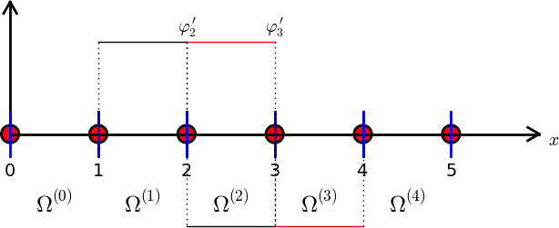
Let's choose the obvious finite element basis: $ \baspsi_i=\basphi_i $, $ i=0,\ldots,N_n-1 $

Problem: $ \basphi_0(0)\neq 0 $ and $ \basphi_{N_n-1}(L)\neq 0 $

Solution: we just exclude $ \basphi_0 $ and $ \basphi_{N_n-1} $ from the basis and work with $$ \baspsi_i=\basphi_{i+1},\quad i=0,\ldots,N=N_n-3$$

Introduce index mapping $ \nu(i) $: $ \baspsi_i = \basphi_{\nu(i)} $ $$ u = \sum_{j\in\If}c_j\basphi_{\nu(j)},\quad i=0,\ldots,N,\quad \nu(j) = j+1$$

Irregular numbering: more complicated $ \nu(j) $ table

Computation in the global physical domain; formulas

$$ \begin{equation*} A_{i,j}=\int_0^L\basphi_{i+1}'(x)\basphi_{j+1}'(x) dx,\quad b_i=\int_0^L2\basphi_{i+1}(x) dx \end{equation*} $$

Many will prefer to change indices to obtain a $ \basphi_i'\basphi_j' $ product: $ i+1\rightarrow i $, $ j+1\rightarrow j $ $$ \begin{equation*} A_{i-1,j-1}=\int_0^L\basphi_{i}'(x)\basphi_{j}'(x) \dx,\quad b_{i-1}=\int_0^L2\basphi_{i}(x) \dx \end{equation*} $$

Computation in the global physical domain; details

$$ \basphi_i' \sim \pm h^{-1} $$ $$ A_{i-1,i-1} = h^{-2}2h = 2h^{-1},\quad A_{i-1,i-2} = h^{-1}(-h^{-1})h = -h^{-1}$$ and $ A_{i-1,i}=A_{i-1,i-2} $ $$ b_{i-1} = 2({\half}h + {\half}h) = 2h$$

Computation in the global physical domain; linear system

$$ \begin{equation*} { \frac{1}{h}\left( \begin{array}{ccccccccc} 2 & -1 & 0 &\cdots & \cdots & \cdots & \cdots & \cdots & 0 \\ -1 & 2 & -1 & \ddots & & & & & \vdots \\ 0 & -1 & 2 & -1 & \ddots & & & & \vdots \\ \vdots & \ddots & & \ddots & \ddots & 0 & & & \vdots \\ \vdots & & \ddots & \ddots & \ddots & \ddots & \ddots & & \vdots \\ \vdots & & & 0 & -1 & 2 & -1 & \ddots & \vdots \\ \vdots & & & & \ddots & \ddots & \ddots &\ddots & 0 \\ \vdots & & & & &\ddots & \ddots &\ddots & -1 \\ 0 &\cdots & \cdots &\cdots & \cdots & \cdots & 0 & -1 & 2 \end{array} \right) \left( \begin{array}{c} c_0 \\ \vdots\\ \vdots\\ \vdots \\ \vdots \\ \vdots \\ \vdots \\ \vdots\\ c_{N} \end{array} \right) = \left( \begin{array}{c} 2h \\ \vdots\\ \vdots\\ \vdots \\ \vdots \\ \vdots \\ \vdots \\ \vdots\\ 2h \end{array} \right) } \end{equation*} $$

Write out the corresponding difference equation

General equation at node $ i $: $$ -\frac{1}{h}c_{i-1} + \frac{2}{h}c_{i} - \frac{1}{h}c_{i+1} = 2h $$

Now, $ c_i = u(\xno{i+1})\equiv u_{i+1} $. Writing out the equation at node $ i-1 $, $$ -\frac{1}{h}c_{i-2} + \frac{2}{h}c_{i-1} - \frac{1}{h}c_{i} = 2h $$

translates directly to $$ -\frac{1}{h}u_{i-1} + \frac{2}{h}u_{i} - \frac{1}{h}u_{i+1} = 2h $$

Comparison with a finite difference discretization

The standard finite difference method for $ -u''=2 $ is $$ -\frac{1}{h^2}u_{i-1} + \frac{2}{h^2}u_{i} - \frac{1}{h^2}u_{i+1} = 2 $$

Multiply by $ h $!

The finite element method and the finite difference method are identical in this example.

(Remains to study the equations at the end points, which involve boundary values - but these are also the same for the two methods)

Cellwise computations; formulas

Repeat the previous example, but apply the cellwise algorithm

Work with one cell at a time

Transform physical cell to reference cell $ X\in [-1,1] $

$$ \begin{equation*} A_{i-1,j-1}^{(e)}=\int_{\Omega^{(e)}} \basphi_i'(x)\basphi_j'(x) \dx = \int_{-1}^1 \frac{d}{dx}\refphi_r(X)\frac{d}{dx}\refphi_s(X) \frac{h}{2} \dX, \end{equation*} $$ $$ \refphi_0(X)=\half(1-X),\quad\refphi_1(X)=\half(1+X)$$ $$ \frac{d\refphi_0}{dX} = -\half,\quad \frac{d\refphi_1}{dX} = \half $$

From the chain rule $$ \frac{d\refphi_r}{dx} = \frac{d\refphi_r}{dX}\frac{dX}{dx} = \frac{2}{h}\frac{d\refphi_r}{dX}$$

Cellwise computations; details

$$ \begin{equation*} A_{i-1,j-1}^{(e)}=\int_{\Omega^{(e)}} \basphi_i'(x)\basphi_j'(x) \dx = \int_{-1}^1 \frac{2}{h}\frac{d\refphi_r}{dX}\frac{2}{h}\frac{d\refphi_s}{dX} \frac{h}{2} \dX = \tilde A_{r,s}^{(e)} \end{equation*} $$ $$ \begin{equation*} b_{i-1}^{(e)} = \int_{\Omega^{(e)}} 2\basphi_i(x) \dx = \int_{-1}^12\refphi_r(X)\frac{h}{2} \dX = \tilde b_{r}^{(e)}, \quad i=q(e,r),\ r=0,1 \end{equation*} $$

Must run through all $ r,s=0,1 $ and $ r=0,1 $ and compute each entry in the element matrix and vector: $$ \begin{equation*} \tilde A^{(e)} =\frac{1}{h}\left(\begin{array}{rr} 1 & -1\\ -1 & 1 \end{array}\right),\quad \tilde b^{(e)} = h\left(\begin{array}{c} 1\\ 1 \end{array}\right) \end{equation*} $$

Example: $$ \tilde A^{(e)}_{0,1} = \int_{-1}^1 \frac{2}{h}\frac{d\refphi_0}{dX}\frac{2}{h}\frac{d\refphi_1}{dX} \frac{h}{2} \dX = \frac{2}{h}(-\half)\frac{2}{h}\half\frac{h}{2} \int_{-1}^1\dX = -\frac{1}{h} $$

Cellwise computations; details of boundary cells

The boundary cells involve only one unknown

$ \Omega^{(0)} $: left node value known, only a contribution from right node

$ \Omega^{(N_e)} $: right node value known, only a contribution from left node

For $ e=0 $ and $ =N_e $: $$ \tilde A^{(e)} =\frac{1}{h}\left(\begin{array}{r} 1 \end{array}\right),\quad \tilde b^{(e)} = h\left(\begin{array}{c} 1 \end{array}\right) $$

Only one degree of freedom ("node") in these cells ($ r=0 $ counts the only dof)

Cellwise computations; assembly

4 P1 elements:

1 2 3
vertices = [0, 0.5, 1, 1.5, 2] cells = [[0, 1], [1, 2], [2, 3], [3, 4]] dof_map = [[0], [0, 1], [1, 2], [2]] # only 1 dof in elm 0, 3

Python code for the assembly algorithm:

1 2 3 4 5 6 7 8
# Ae[e][r,s]: element matrix, be[e][r]: element vector # A[i,j]: coefficient matrix, b[i]: right-hand side for e in range(len(Ae)): for r in range(Ae[e].shape[0]): for s in range(Ae[e].shape[1]): A[dof_map[e,r],dof_map[e,s]] += Ae[e][i,j] b[dof_map[e,r]] += be[e][i,j]

Result: same linear system as arose from computations in the physical domain

General construction of a boundary function

Now we address nonzero Dirichlet conditions

$ B(x) $ is not always easy to construct (i.e., extend to the interior of $ \Omega $), especially not in 2D and 3D

With finite element basis functions, $ \basphi_i $, $ B(x) $ can be constructed in a completely general way (!)

Define

$ \Ifb $: set of indices with nodes where $ u $ is known

$ U_i $: Dirichlet value of $ u $ at node $ i $, $ i\in\Ifb $

The general formula for $ B $ is now $$ \begin{equation*} B(x) = \sum_{j\in\Ifb} U_j\basphi_j(x) \end{equation*} $$

Explanation

Suppose we have a Dirichlet condition $ u(\xno{k})=U_k $, $ k\in\Ifb $: $$ u(\xno{k}) = \sum_{j\in\Ifb} U_j\underbrace{\basphi_j(x_k)}_{\neq 0 \hbox{ only for }j=k} + \sum_{j\in\If} c_j\underbrace{\basphi_{\nu(j)}(\xno{k})}_{=0,\ k\not\in\If} = U_k $$

Example with two nonzero Dirichlet values; variational formulation

$$ -u''=2, \quad u(0)=C,\ u(L)=D $$ $$ \int_0^L u'v'\dx = \int_0^L2v\dx\quad\forall v\in V$$ $$ (u',v') = (2,v)\quad\forall v\in V$$

Example with two Dirichlet values; boundary function

$$ \begin{equation*} B(x) = \sum_{j\in\Ifb} U_j\basphi_j(x) \end{equation*} $$

Here $ \Ifb = \{0,N_n-1\} $, $ U_0=C $, $ U_{N_n-1}=D $; $ \baspsi_i $ are the internal $ \basphi_i $ functions: $$ \baspsi_i = \basphi_{\nu(i)}, \quad \nu(i)=i+1,\quad i\in\If = \{0,\ldots,N=N_n-3\} $$ $$ \begin{align*} u(x) &= \underbrace{C\basphi_0 + D\basphi_{N_n-1}}_{B(x)} + \sum_{j\in\If} c_j\basphi_{j+1}\\ &= C\basphi_0 + D\basphi_{N_n-1} + c_0\basphi_1 + c_1\basphi_2 +\cdots + c_N\basphi_{N_n-2} \end{align*} $$

Example with two Dirichlet values; details

Insert $ u = B + \sum_j c_j\baspsi_j $ in variational formulation: $$ (u',v') = (2,v)\quad\Rightarrow\quad (\sum_jc_j\baspsi_j',\baspsi_i') = (2,\baspsi_i)-(B',\baspsi_i')\quad \forall v\in V$$ $$ \begin{align*} A_{i-1,j-1} &= \int_0^L \basphi_i'(x)\basphi_j'(x) \dx\\ b_{i-1} &= \int_0^L (f(x)\basphi_i(x) - B'(x)\basphi_i'(x))\dx,\quad B'(x)=C\basphi_{0}'(x) + D\basphi_{N_n-1}'(x) \end{align*} $$ for $ i,j = 1,\ldots,N+1=N_n-2 $.

New boundary terms from $ -\int B'\basphi_i'\dx $: add $ C/h $ to $ b_0 $ and $ D/h $ to $ b_N $

Example with two Dirichlet values; cellwise computations

All element matrices are as in the previous example

New element vector in the first and last cell

From the first cell: $$ \tilde b_0^{(1)} = \int_{-1}^1 \left(f\refphi_1 - C\frac{2}{h}\frac{d\refphi_0}{dX}\frac{2}{h}\frac{d\refphi_1}{dX}\right) \frac{h}{2} \dX = \frac{h}{2} 2\int_{-1}^1 \refphi_1 \dX - C\frac{2}{h}(-\frac{1}{2})\frac{2}{h}\frac{1}{2}\frac{h}{2}\cdot 2 = h + C\frac{1}{h}\tp $$

From the last cell: $$ \tilde b_0^{(N_e)} = \int_{-1}^1 \left(f\refphi_0 - D\frac{2}{h}\frac{d\refphi_1}{dX}\frac{2}{h}\frac{d\refphi_0}{dX}\right) \frac{h}{2} \dX = \frac{h}{2} 2\int_{-1}^1 \refphi_0 \dX - D\frac{2}{h}\frac{1}{2}\frac{2}{h}(-\frac{1}{2})\frac{h}{2}\cdot 2 = h + D\frac{1}{h}\tp $$

Modification of the linear system; ideas

Method 1: incorporate Dirichlet values through a $ B(x) $ function and demand $ \baspsi_i=0 $ where Dirichlet values apply

Method 2: drop $ B(x) $, drop demands to $ \baspsi_i $, just assemble as if there were no Dirichlet conditions, and modify the linear system instead

Method 2: always choose $ \baspsi_i = \basphi_i $ for all $ i\in\If $ and set $$ \begin{equation*} u(x) = \sum_{j\in\If}c_j\basphi_j(x),\quad \If=\{0,\ldots,N=N_n-1\} \end{equation*} $$

Attractive way of incorporating Dirichlet conditions.

$ u $ is treated as unknown at all boundaries when computing entries in the linear system

Modification of the linear system; original system

$$ -u''=2,\quad u(0)=0,\ u(L)=D$$

Assemble as if there were no Dirichlet conditions: $$ \begin{equation*} { \frac{1}{h}\left( \begin{array}{ccccccccc} 1 & -1 & 0 &\cdots & \cdots & \cdots & \cdots & \cdots & 0 \\ -1 & 2 & -1 & \ddots & & & & & \vdots \\ 0 & -1 & 2 & -1 & \ddots & & & & \vdots \\ \vdots & \ddots & & \ddots & \ddots & 0 & & & \vdots \\ \vdots & & \ddots & \ddots & \ddots & \ddots & \ddots & & \vdots \\ \vdots & & & 0 & -1 & 2 & -1 & \ddots & \vdots \\ \vdots & & & & \ddots & \ddots & \ddots &\ddots & 0 \\ \vdots & & & & &\ddots & \ddots &\ddots & -1 \\ 0 &\cdots & \cdots &\cdots & \cdots & \cdots & 0 & -1 & 1 \end{array} \right) \left( \begin{array}{c} c_0 \\ \vdots\\ \vdots\\ \vdots \\ \vdots \\ \vdots \\ \vdots \\ \vdots\\ c_{N} \end{array} \right) = \left( \begin{array}{c} h \\ 2h\\ \vdots\\ \vdots \\ \vdots \\ \vdots \\ \vdots \\ 2h\\ h \end{array} \right) } \end{equation*} $$

Modification of the linear system; row replacement

Dirichlet condition $ u(\xno{k})= U_k $ means $ c_k=U_k $
(since $ c_k=u(\xno{k}) $)

Replace first row by $ c_0=0 $

Replace last row by $ c_N=D $

$$ \begin{equation*} { \frac{1}{h}\left( \begin{array}{ccccccccc} h & 0 & 0 &\cdots & \cdots & \cdots & \cdots & \cdots & 0 \\ -1 & 2 & -1 & \ddots & & & & & \vdots \\ 0 & -1 & 2 & -1 & \ddots & & & & \vdots \\ \vdots & \ddots & & \ddots & \ddots & 0 & & & \vdots \\ \vdots & & \ddots & \ddots & \ddots & \ddots & \ddots & & \vdots \\ \vdots & & & 0 & -1 & 2 & -1 & \ddots & \vdots \\ \vdots & & & & \ddots & \ddots & \ddots &\ddots & 0 \\ \vdots & & & & &\ddots & \ddots &\ddots & -1 \\ 0 &\cdots & \cdots &\cdots & \cdots & \cdots & 0 & 0 & h \end{array} \right) \left( \begin{array}{c} c_0 \\ \vdots\\ \vdots\\ \vdots \\ \vdots \\ \vdots \\ \vdots \\ \vdots\\ c_{N} \end{array} \right) = \left( \begin{array}{c} 0 \\ 2h\\ \vdots\\ \vdots \\ \vdots \\ \vdots \\ \vdots \\ 2h\\ D \end{array} \right) } \end{equation*} $$

Modification of the linear system; element matrix/vector

In cell 0 we know $ u $ for local node (degree of freedom) $ r=0 $. Replace the first cell equation by $ \tilde c_0 = 0 $: $$ \begin{equation*} \tilde A^{(0)} = A = \frac{1}{h}\left(\begin{array}{rr} h & 0\\ -1 & 1 \end{array}\right),\quad \tilde b^{(0)} = \left(\begin{array}{c} 0\\ h \end{array}\right) \end{equation*} $$

In cell $ N_e $ we know $ u $ for local node $ r=1 $. Replace the last equation in the cell system by $ \tilde c_1=D $: $$ \begin{equation*} \tilde A^{(N_e)} = A = \frac{1}{h}\left(\begin{array}{rr} 1 & -1\\ 0 & h \end{array}\right),\quad \tilde b^{(N_e)} = \left(\begin{array}{c} h\\ D \end{array}\right) \end{equation*} $$

Symmetric modification of the linear system; algorithm

The modification above destroys symmetry of the matrix: e.g., $ A_{0,1}\neq A_{1,0} $

Symmetry is often important in 2D and 3D
(faster computations, less storage)

A more complex modification can preserve symmetry!

Algorithm for incorporating $ c_i=U_i $ in a symmetric way:

Subtract column $ i $ times $ U_i $ from the right-hand side

Zero out column and row no $ i $

Place 1 on the diagonal

Set $ b_i=U_i $

Symmetric modification of the linear system; example

$$ \begin{equation*} { \frac{1}{h}\left( \begin{array}{ccccccccc} h & 0 & 0 &\cdots & \cdots & \cdots & \cdots & \cdots & 0 \\ 0 & 2 & -1 & \ddots & & & & & \vdots \\ 0 & -1 & 2 & -1 & \ddots & & & & \vdots \\ \vdots & \ddots & & \ddots & \ddots & 0 & & & \vdots \\ \vdots & & \ddots & \ddots & \ddots & \ddots & \ddots & & \vdots \\ \vdots & & & 0 & -1 & 2 & -1 & \ddots & \vdots \\ \vdots & & & & \ddots & \ddots & \ddots &\ddots & 0 \\ \vdots & & & & &\ddots & \ddots &\ddots & 0 \\ 0 &\cdots & \cdots &\cdots & \cdots & \cdots & 0 & 0 & h \end{array} \right) \left( \begin{array}{c} c_0 \\ \vdots\\ \vdots\\ \vdots \\ \vdots \\ \vdots \\ \vdots \\ \vdots\\ c_{N} \end{array} \right) = \left( \begin{array}{c} 0 \\ 2h\\ \vdots\\ \vdots \\ \vdots \\ \vdots \\ \vdots \\ 2h +\frac{D}{h}\\ D \end{array} \right) } \end{equation*} $$

Symmetric modification of the linear system; element level

Symmetric modification applied to $ \tilde A^{(N_e)} $: $$ \begin{equation*} \tilde A^{(N_e)} = A = \frac{1}{h}\left(\begin{array}{rr} 1 & 0\\ 0 & h \end{array}\right),\quad \tilde b^{(N_e)} = \left(\begin{array}{c} h + D/h\\ D \end{array}\right) \end{equation*} $$

Boundary conditions: specified derivative

Neumann conditions.

How can we incorporate $ u'(0)=C $ with finite elements?

$$ -u''=f,\quad u'(0)=C,\ u(L)=D$$

$ \baspsi_i(L)=0 $ because of Dirichlet condition $ u(L)=D $
(or no demand and modify linear system)

No demand to $ \baspsi_i(0) $

The condition $ u'(0)=C $ will be handled (as usual) through a boundary term arising from integration by parts

The variational formulation

Galerkin's method: $$ \begin{equation*} \int_0^L(u''(x)+f(x))\baspsi_i(x) dx = 0,\quad i\in\If \end{equation*} $$

Integration of $ u''\baspsi_i $ by parts: $$ \begin{equation*} \int_0^Lu'(x)\baspsi_i'(x) \dx -(u'(L)\baspsi_i(L) - u'(0)\baspsi_i(0)) - \int_0^L f(x)\baspsi_i(x) \dx =0 \end{equation*} $$

$ u'(L){\baspsi_i(L)}=0 $ since $ \baspsi_i(L)=0 $

$ u'(0)\baspsi_i(0) = C\baspsi_i(0) $ since $ u'(0)=C $

Method 1: Boundary function and exclusion of Dirichlet degrees of freedom

$ \baspsi_i = \basphi_i $, $ i\in\If =\{0,\ldots,N=N_n-2\} $

$ B(x)=D\basphi_{N_n-1}(x) $, $ u= B + \sum_{j=0}^N c_j\basphi_j $

$$ \begin{equation*} \int_0^Lu'(x)\basphi_i'(x) dx = \int_0^L f(x)\basphi_i(x) dx - C\basphi_i(0),\quad i\in\If \end{equation*} $$ $$ \begin{equation*} \sum_{j=0}^{N}\left( \int_0^L \basphi_i'\basphi_j' dx \right)c_j = \int_0^L\left(f\basphi_i -D\basphi_N'\basphi_i\right) dx - C\basphi_i(0) \end{equation*} $$ for $ i=0,\ldots,N=N_n-2 $.

Method 2: Use all $ \basphi_i $ and insert the Dirichlet condition in the linear system

Now $ \baspsi_i=\basphi_i $, $ i=0,\ldots,N=N_n-1 $ (all nodes)

$ \basphi_N(L)\neq 0 $, so $ u'(L)\basphi_N(L)\neq 0 $

However, the term $ u'(L)\basphi_N(L) $ in $ b_N $ will be erased when we insert the Dirichlet value in $ b_N=D $

We can therefore forget about the term $ u'(L)\basphi_i(L) $!

Boundary terms $ u'\basphi_i $ at points $ \xno{i} $ where Dirichlet values apply can always be forgotten.

$$ \begin{equation*} u(x) = \sum_{j=0}^{N=N_n-1} c_j\basphi_j(x) \end{equation*} $$ $$ \begin{equation*} \sum_{j=0}^{N=N_n-1}\left( \int_0^L \basphi_i'(x)\basphi_j'(x) dx \right)c_j = \int_0^L f(x)\basphi_i(x) dx - C\basphi_i(0) \end{equation*} $$

Assemble entries for $ i=0,\ldots,N=N_n-1 $ and then modify the last equation to $ c_N=D $

How the Neumann condition impacts the element matrix and vector

The extra term $ C\basphi_0(0) $ affects only the element vector from the first cell since $ \basphi_0=0 $ on all other cells. $$ \begin{equation*} \tilde A^{(0)} = A = \frac{1}{h}\left(\begin{array}{rr} 1 & 1\\ -1 & 1 \end{array}\right),\quad \tilde b^{(0)} = \left(\begin{array}{c} h - C\\ h \end{array}\right) \end{equation*} $$

The finite element algorithm

The differential equation problem defines the integrals in the variational formulation.

Request these functions from the user:

1 2 3 4
integrand_lhs(phi, r, s, x) boundary_lhs(phi, r, s, x) integrand_rhs(phi, r, x) boundary_rhs(phi, r, x)

Must also have a mesh with vertices, cells, and dof_map

Python pseudo code; the element matrix and vector

1 2 3 4 5 6 7 8 9 10 11 12 13 14 15 16 17 18 19 20 21 22 23 24 25 26
<Declare global matrix, global rhs: A, b> # Loop over all cells for e in range(len(cells)): # Compute element matrix and vector n = len(dof_map[e]) # no of dofs in this element h = vertices[cells[e][1]] - vertices[cells[e][0]] <Declare element matrix, element vector: A_e, b_e> # Integrate over the reference cell points, weights = <numerical integration rule> for X, w in zip(points, weights): phi = <basis functions + derivatives at X> detJ = h/2 x = <affine mapping from X> for r in range(n): for s in range(n): A_e[r,s] += integrand_lhs(phi, r, s, x)*detJ*w b_e[r] += integrand_rhs(phi, r, x)*detJ*w # Add boundary terms for r in range(n): for s in range(n): A_e[r,s] += boundary_lhs(phi, r, s, x)*detJ*w b_e[r] += boundary_rhs(phi, r, x)*detJ*w

Python pseudo code; boundary conditions and assembly

1 2 3 4 5 6 7 8 9 10 11 12 13 14 15 16 17 18 19 20 21 22 23
for e in range(len(cells)): ... # Incorporate essential boundary conditions for r in range(n): global_dof = dof_map[e][r] if global_dof in essbc_dofs: # dof r is subject to an essential condition value = essbc_docs[global_dof] # Symmetric modification b_e -= value*A_e[:,r] A_e[r,:] = 0 A_e[:,r] = 0 A_e[r,r] = 1 b_e[r] = value # Assemble for r in range(n): for s in range(n): A[dof_map[e][r], dof_map[e][r]] += A_e[r,s] b[dof_map[e][r] += b_e[r] <solve linear system>

Variational formulations in 2D and 3D

Major differences when going from 1D to 2D/3D.

The integration by part formula is different

Cells have different geometry

Integration by parts

Rule for multi-dimensional integration by parts.

$$ \begin{equation*} -\int_{\Omega} \nabla\cdot (\dfc(\x)\nabla u) v\dx = \int_{\Omega} \dfc(\x)\nabla u\cdot\nabla v \dx - \int_{\partial\Omega} a\frac{\partial u}{\partial n} v \ds \end{equation*} $$

$ \int_\Omega ()\dx $: area (2D) or volume (3D) integral

$ \int_{\partial\Omega} ()\ds $: line(2D) or surface (3D) integral

$ \partial\Omega_N $: Neumann conditions $ -a\frac{\partial u}{\partial n} = g $

$ \partial\Omega_D $: Dirichlet conditions $ u = u_0 $

$ v\in V $ must vanish on $ \partial\Omega_D $ (in method 1)

Example on integration by parts; problem

$$ \begin{align*} \v\cdot\nabla u + \beta u &= \nabla\cdot\left( \dfc\nabla u\right) + f, \quad & \x\in\Omega\\ u &= u_0,\quad &\x\in\partial\Omega_D\\ -\dfc\frac{\partial u}{\partial n} &= g,\quad &\x\in\partial\Omega_N \end{align*} $$

Known: $ \dfc $, $ \beta $, $ f $, $ u_0 $, and $ g $.

Second-order PDE: must have exactly one boundary condition at each point of the boundary

Method 1 with boundary function and $ \baspsi_i=0 $ on $ \partial\Omega_D $ (ensures $ u=u_0 $ condition): $$ u(\x) = B(\x) + \sum_{j\in\If} c_j\baspsi_j(\x),\quad B(\x)=u_0(\x) $$

Example on integration by parts in 1D/2D/3D

Galerkin's method: multiply by $ v\in V $ and integrate over $ \Omega $, $$ \int_{\Omega} (\v\cdot\nabla u + \beta u)v\dx = \int_{\Omega} \nabla\cdot\left( \dfc\nabla u\right)v\dx + \int_{\Omega}fv \dx $$

Integrate the second-order term by parts according to the formula: $$ \int_{\Omega} \nabla\cdot\left( \dfc\nabla u\right) v \dx = -\int_{\Omega} \dfc\nabla u\cdot\nabla v\dx + \int_{\partial\Omega} \dfc\frac{\partial u}{\partial n} v\ds, $$

Galerkin's method then gives $$ \int_{\Omega} (\v\cdot\nabla u + \beta u)v\dx = -\int_{\Omega} \dfc\nabla u\cdot\nabla v\dx + \int_{\partial\Omega} \dfc\frac{\partial u}{\partial n} v\ds + \int_{\Omega} fv \dx $$

Incorporation of the Neumann condition in the variational formulation

Note: $ v\neq 0 $ only on $ \partial\Omega_N $ (since $ v=0 $ on $ \partial\Omega_D $): $$ \int_{\partial\Omega} \dfc\frac{\partial u}{\partial n} v\ds = \int_{\partial\Omega_N} \underbrace{\dfc\frac{\partial u}{\partial n}}_{-g} v\ds = -\int_{\partial\Omega_N} gv\ds $$

The final variational form: $$ \int_{\Omega} (\v\cdot\nabla u + \beta u)v\dx = -\int_{\Omega} \dfc\nabla u\cdot\nabla v \dx - \int_{\partial\Omega_N} g v\ds + \int_{\Omega} fv \dx $$

Or with inner product notation: $$ (\v\cdot\nabla u, v) + (\beta u,v) = - (\dfc\nabla u,\nabla v) - (g,v)_{N} + (f,v) $$

$ (g,v)_{N} $: line or surface integral over $ \partial\Omega_N $.

Derivation of the linear system

$ \forall v\in V $ is replaced by for all $ \baspsi_i $, $ i\in\If $

Insert $ u = B + \sum_{j\in\If} c_j\baspsi_j $, $ B = u_0 $, in the variational form

Identify $ i,j $ terms (matrix) and $ i $ terms (right-hand side)

Write on form $ \sum_{i\in\If}A_{i,j}c_j = b_i $, $ i\in\If $

$$ A_{i,j} = (\v\cdot\nabla \baspsi_j, \baspsi_i) + (\beta \baspsi_j ,\baspsi_i) + (\dfc\nabla \baspsi_j,\nabla \baspsi_i) $$ $$ b_i = (g,\baspsi_i)_{N} + (f,\baspsi_i) - (\v\cdot\nabla u_0, \baspsi_i) + (\beta u_0 ,\baspsi_i) + (\dfc\nabla u_0,\nabla \baspsi_i) $$

Transformation to a reference cell in 2D/3D (1)

We want to compute an integral in the physical domain by integrating over the reference cell.

$$ \begin{equation*} \int_{{\Omega}^{(e)}} \dfc(\x)\nabla\basphi_i\cdot\nabla\basphi_j\dx \end{equation*} $$

Mapping from reference to physical coordinates: $$ \x(\X) $$

with Jacobian $ J $, $$ J_{i,j}=\frac{\partial x_j}{\partial X_i} $$

Transformation to a reference cell in 2D/3D (2)

$ \dx \rightarrow \det J\dX $.

Must express $ \nabla\basphi_i $ by an expression with $ \refphi_r $, $ i=q(e,r) $: $ \nabla\refphi_r(\X) $

We want $ \nabla_{\x}\refphi_r(\X) $ (derivatives wrt $ \x $)

What we readily have is $ \nabla_{\X}\refphi_r(\X) $ (derivative wrt $ \X $)

Need to transform $ \nabla_{\X}\refphi_r(\X) $ to $ \nabla_{\x}\refphi_r(\X) $

Transformation to a reference cell in 2D/3D (3)

Can derive $$ \begin{align*} \nabla_{\X}\refphi_r &= J\cdot\nabla_{\x}\basphi_i\\ \nabla_{\x}\basphi_i &= \nabla_{\x}\refphi_r(\X) = J^{-1}\cdot\nabla_{\X}\refphi_r(\X) \end{align*} $$

Integral transformation from physical to reference coordinates: $$ \begin{equation*} \int_{\Omega^{(e)}} \dfc(\x)\nabla_{\x}\basphi_i\cdot\nabla_{\x}\basphi_j\dx = \int_{\tilde\Omega^r} \dfc(\x(\X))(J^{-1}\cdot\nabla_{\X}\refphi_r)\cdot (J^{-1}\cdot\nabla\refphi_s)\det J\dX \end{equation*} $$

Numerical integration

Numerical integration over reference cell triangles and tetrahedra: $$ \int_{\tilde\Omega^r} g\dX = \sum_{j=0}^{n-1} w_j g(\bar\X_j)$$

Module numint.py contains different rules:

1 2 3 4 5 6 7 8
>>> import numint >>> x, w = numint.quadrature_for_triangles(num_points=3) >>> x [(0.16666666666666666, 0.16666666666666666), (0.66666666666666666, 0.16666666666666666), (0.16666666666666666, 0.66666666666666666)] >>> w [0.16666666666666666, 0.16666666666666666, 0.16666666666666666]

Triangle: rules with $ n=1,3,4,7 $ integrate exactly polynomials of degree $ 1,2,3,4 $, resp.

Tetrahedron: rules with $ n=1,4,5,11 $ integrate exactly polynomials of degree $ 1,2,3,4 $, resp.

Study guide: Computing with variational forms

2016

Table of contents

Basic principles for approximating differential equations

We shall apply least squares, Galerkin/projection, and collocation to differential equation models

Abstract differential equation

Abstract boundary conditions

Reminder about notation

New topics: variational formulation and boundary conditions

Residual-minimizing principles

The least squares method

The Galerkin method

The Method of Weighted Residuals

New terminology: test and trial functions

The collocation method

Examples on using the principles

The first model problem

Boundary conditions

The least squares method; principle

The least squares method; equation system

The least squares method; matrix and right-hand side expressions

Orthogonality of the basis functions gives diagonal matrix

Least squares method; solution

The Galerkin method; principle

The Galerkin method; solution

The collocation method

Comparison of the methods

Useful techniques

Integration by parts has many advantages

We use a boundary function to deal with non-zero Dirichlet boundary conditions

Example on constructing a boundary function for two Dirichlet conditions

Example on constructing a boundary function for one Dirichlet condition

With a \( B(x) \), \( u\not\in V \), but \( \sum_{j}c_j\baspsi_j\in V \)

Abstract notation for variational formulations

Example on abstract notation

Bilinear and linear forms

The linear system associated with the abstract form

Equivalence with minimization problem

Examples on variational formulations

Variable coefficient; problem

Variable coefficient; Galerkin principle

Variable coefficient; integration by parts

Variable coefficient; variational formulation

Variable coefficient; linear system (the easy way)

Variable coefficient; linear system (full derivation)

First-order derivative in the equation and boundary condition; problem

First-order derivative in the equation and boundary condition; details

First-order derivative in the equation and boundary condition; observations

First-order derivative in the equation and boundary condition; abstract notation (optional)

First-order derivative in the equation and boundary condition; linear system

Terminology: natural and essential boundary conditions

Nonlinear coefficient; problem

Nonlinear coefficient; variational formulation

Nonlinear coefficient; where does the nonlinearity cause challenges?

Examples on detailed computations by hand

Dirichlet and Neumann conditions; problem

Dirichlet and Neumann conditions; linear system

Dirichlet and Neumann conditions; integration

Dirichlet and Neumann conditions; \( 2\times 2 \) system

When the numerical method is exact?

Computing with finite elements

Variational formulation

How to deal with the boundary conditions?

Computation in the global physical domain; formulas

Computation in the global physical domain; details

Computation in the global physical domain; linear system

Write out the corresponding difference equation

Comparison with a finite difference discretization

Cellwise computations; formulas

Cellwise computations; details

Cellwise computations; details of boundary cells

Cellwise computations; assembly

General construction of a boundary function

Explanation

Example with two nonzero Dirichlet values; variational formulation

Example with two Dirichlet values; boundary function

Example with two Dirichlet values; details

Example with two Dirichlet values; cellwise computations

Modification of the linear system; ideas

Modification of the linear system; original system