Basic principles for approximating differential equations

We shall apply least squares, Galerkin/projection, and collocation to differential equation models

Our aim is to extend the ideas for approximating \( f \) by \( u \), or solving

 
$$ u = f $$

to real, spatial differential equations like

 
$$ -u'' + bu = f,\quad u(0)=C,\ u'(L)=D $$

Abstract differential equation

 
$$ \begin{equation*} \mathcal{L}(u) = 0,\quad x\in\Omega \end{equation*} $$

Examples (1D problems):

 
$$ \begin{align*} \mathcal{L}(u) &= \frac{d^2u}{dx^2} - f(x),\\ \mathcal{L}(u) &= \frac{d}{dx}\left(\dfc(x)\frac{du}{dx}\right) + f(x),\\ \mathcal{L}(u) &= \frac{d}{dx}\left(\dfc(u)\frac{du}{dx}\right) - au + f(x),\\ \mathcal{L}(u) &= \frac{d}{dx}\left(\dfc(u)\frac{du}{dx}\right) + f(u,x) \end{align*} $$

Abstract boundary conditions

 
$$ \begin{equation*} \mathcal{B}_0(u)=0,\ x=0,\quad \mathcal{B}_1(u)=0,\ x=L \end{equation*} $$

Examples:

 
$$ \begin{align*} \mathcal{B}_i(u) &= u - g,\quad &\hbox{Dirichlet condition}\\ \mathcal{B}_i(u) &= -\dfc \frac{du}{dx} - g,\quad &\hbox{Neumann condition}\\ \mathcal{B}_i(u) &= -\dfc \frac{du}{dx} - h(u-g),\quad &\hbox{Robin condition} \end{align*} $$

Reminder about notation

• \( \uex(x) \) is the symbol for the exact solution of \( \mathcal{L}(\uex)=0 \) and \( \mathcal{B}_i (\uex)=0 \)
• \( u(x) \) denotes an approximate solution
• \( V = \hbox{span}\{ \baspsi_0(x),\ldots,\baspsi_N(x)\} \), \( V \) has basis \( \sequencei{\baspsi} \)
• We seek \( u\in V \)
• \( \If =\{0,\ldots,N\} \) is an index set
• \( u(x) = \sum_{j\in\If} c_j\baspsi_j(x) \)
• Inner product: \( (u,v) = \int_\Omega uv\dx \)
• Norm: \( ||u||=\sqrt{(u,u)} \)

New topics: variational formulation and boundary conditions

Much is similar to approximating a function (solving \( u=f \)), but two new topics are needed:

• Variational formulation of the differential equation problem (including integration by parts)
• Handling of boundary conditions

Residual-minimizing principles

• When solving \( u=f \) we knew the error \( e=f-u \) and could use principles for minimizing the error
• When solving \( \mathcal{L}(\uex)=0 \) we do not know \( \uex \) and cannot work with the error \( e=\uex - u \)
• We can only know the error in the equation: the residual \( R \)

Inserting \( u=\sum_jc_j\baspsi_j \) in \( \mathcal{L}=0 \) gives a residual \( R \)

 
$$ \begin{equation*} \mathcal{L}(u) = \mathcal{L}(\sum_j c_j \baspsi_j) = R \neq 0 \end{equation*} $$

Goal: minimize \( R \) with respect to \( \sequencei{c} \) (and hope it makes a small \( e \) too)

 
$$ R=R(c_0,\ldots,c_N; x)$$

The least squares method

Idea: minimize

 
$$ \begin{equation*} E = ||R||^2 = (R,R) = \int_{\Omega} R^2 dx \end{equation*} $$

Minimization wrt \( \sequencei{c} \) implies

 
$$ \frac{\partial E}{\partial c_i} = \int_{\Omega} 2R\frac{\partial R}{\partial c_i} dx = 0\quad \Leftrightarrow\quad (R,\frac{\partial R}{\partial c_i})=0,\quad i\in\If $$

\( N+1 \) equations for \( N+1 \) unknowns \( \sequencei{c} \)

The Galerkin method

Idea: make \( R \) orthogonal to \( V \),

 
$$ (R,v)=0,\quad \forall v\in V $$

This implies

 
$$ (R,\baspsi_i)=0,\quad i\in\If $$

\( N+1 \) equations for \( N+1 \) unknowns \( \sequencei{c} \)

The Method of Weighted Residuals

Generalization of the Galerkin method: demand \( R \) orthogonal to some space \( W \), possibly \( W\neq V \):

 
$$ (R,v)=0,\quad \forall v\in W $$

If \( \{w_0,\ldots,w_N\} \) is a basis for \( W \):

 
$$ (R,w_i)=0,\quad i\in\If $$

• \( N+1 \) equations for \( N+1 \) unknowns \( \sequencei{c} \)
• Weighted residual with \( w_i = \partial R/\partial c_i \) gives least squares

New terminology: test and trial functions

• \( \baspsi_j \) used in \( \sum_jc_j\baspsi_j \) is called trial function
• \( \baspsi_i \) or \( w_i \) used as weight in Galerkin's method is called test function

The collocation method

Idea: demand \( R=0 \) at \( N+1 \) points in space

 
$$ R(\xno{i}; c_0,\ldots,c_N)=0,\quad i\in\If$$

The collocation method is a weighted residual method with delta functions as weights

 
$$ 0 = \int_\Omega R(x;c_0,\ldots,c_N) \delta(x-\xno{i})\dx = R(\xno{i}; c_0,\ldots,c_N)$$

 
$$ \hbox{property of } \delta(x):\quad \int_{\Omega} f(x)\delta (x-\xno{i}) dx = f(\xno{i}),\quad \xno{i}\in\Omega $$

Examples on using the principles

The first model problem

 
$$ -u''(x) = f(x),\quad x\in\Omega=[0,L],\quad u(0)=0,\ u(L)=0$$

Basis functions:

 
$$ \baspsi_i(x) = \sinL{i},\quad i\in\If$$

Residual:

 
$$ \begin{align*} R(x;c_0,\ldots,c_N) &= u''(x) + f(x),\nonumber\\ &= \frac{d^2}{dx^2}\left(\sum_{j\in\If} c_j\baspsi_j(x)\right) + f(x),\nonumber\\ &= \sum_{j\in\If} c_j\baspsi_j''(x) + f(x) \end{align*} $$

Boundary conditions

Since \( u(0)=u(L)=0 \) we must ensure that all \( \baspsi_i(0)=\baspsi_i(L)=0 \), because then

 
$$ u(0) = \sum_jc_j{\color{red}\baspsi_j(0)} = 0,\quad u(L) = \sum_jc_j{\color{red}\baspsi_j(L)} =0 $$

• \( u \) known: Dirichlet boundary condition
• \( u' \) known: Neumann boundary condition
• Must have \( \baspsi_i=0 \) where Dirichlet conditions apply

The least squares method; principle

 
$$ (R,\frac{\partial R}{\partial c_i}) = 0,\quad i\in\If $$

 
$$ \begin{equation*} \frac{\partial R}{\partial c_i} = \frac{\partial}{\partial c_i} \left(\sum_{j\in\If} c_j\baspsi_j''(x) + f(x)\right) = \baspsi_i''(x) \end{equation*} $$

Because:

 
$$ \frac{\partial}{\partial c_i}\left(c_0\baspsi_0'' + c_1\baspsi_1'' + \cdots + c_{i-1}\baspsi_{i-1}'' + {\color{red}c_i\baspsi_{i}''} + c_{i+1}\baspsi_{i+1}'' + \cdots + c_N\baspsi_N'' \right) = \baspsi_{i}'' $$

The least squares method; equation system

 
$$ \begin{equation*} (\sum_j c_j \baspsi_j'' + f,\baspsi_i'')=0,\quad i\in\If \end{equation*} $$

Rearrangement:

 
$$ \begin{equation*} \sum_{j\in\If}(\baspsi_i'',\baspsi_j'')c_j = -(f,\baspsi_i''),\quad i\in\If \end{equation*} $$

This is a linear system

 
$$ \begin{equation*} \sum_{j\in\If}A_{i,j}c_j = b_i,\quad i\in\If \end{equation*} $$

The least squares method; matrix and right-hand side expressions

 
$$ \begin{align*} A_{i,j} &= (\baspsi_i'',\baspsi_j'')\nonumber\\ & = \pi^4(i+1)^2(j+1)^2L^{-4}\int_0^L \sinL{i}\sinL{j}\, dx\nonumber\\ &= \left\lbrace \begin{array}{ll} {1\over2}L^{-3}\pi^4(i+1)^4 & i=j \\ 0, & i\neq j \end{array}\right. \\ b_i &= -(f,\baspsi_i'') = (i+1)^2\pi^2L^{-2}\int_0^Lf(x)\sinL{i}\, dx \end{align*} $$

Orthogonality of the basis functions gives diagonal matrix

Useful property of the chosen basis functions:

 
$$ \begin{equation*} \int\limits_0^L \sinL{i}\sinL{j}\, dx = \delta_{ij},\quad \quad\delta_{ij} = \left\lbrace \begin{array}{ll} \half L & i=j \\ 0, & i\neq j \end{array}\right. \end{equation*} $$

\( \Rightarrow\ (\baspsi_i'',\baspsi_j'') = \delta_{ij} \), i.e., diagonal \( A_{i,j} \), and we can easily solve for \( c_i \):

 
$$ \begin{equation*} c_i = \frac{2L}{\pi^2(i+1)^2}\int_0^Lf(x)\sinL{i}\, dx \end{equation*} $$

Least squares method; solution

Let sympy do the work (\( f(x)=2 \)):

from sympy import *
import sys

i, j = symbols('i j', integer=True)
x, L = symbols('x L')
f = 2
a = 2*L/(pi**2*(i+1)**2)
c_i = a*integrate(f*sin((i+1)*pi*x/L), (x, 0, L))
c_i = simplify(c_i)
print c_i

 
$$ \begin{equation*} c_i = 4 \frac{L^{2} \left(\left(-1\right)^{i} + 1\right)}{\pi^{3} \left(i^{3} + 3 i^{2} + 3 i + 1\right)},\quad u(x) = \sum_{k=0}^{N/2} \frac{8L^2}{\pi^3(2k+1)^3}\sinL{2k} \end{equation*} $$

Fast decay: \( c_2 = c_0/27 \), \( c_4=c_0/125 \) - only one term might be good enough:

 
$$ \begin{equation*} u(x) \approx \frac{8L^2}{\pi^3}\sin\left(\pi\frac{x}{L}\right) \end{equation*} $$

The Galerkin method; principle

\( R=u''+f \):

 
$$ \begin{equation*} (u''+f,v)=0,\quad \forall v\in V, \end{equation*} $$

 
or rearranged,

 
$$ \begin{equation*} (u'',v) = -(f,v),\quad\forall v\in V \end{equation*} $$

This is a variational formulation of the differential equation problem.

\( \forall v\in V \) is equivalent with \( \forall v\in\baspsi_i \), \( i\in\If \), resulting in

 
$$ \begin{equation*} (\sum_{j\in\If} c_j\baspsi_j'', \baspsi_i)=-(f,\baspsi_i),\quad i\in\If \end{equation*} $$

 
$$ \begin{equation*} \sum_{j\in\If}(\baspsi_j'', \baspsi_i) c_j=-(f,\baspsi_i),\quad i\in\If \end{equation*} $$

The Galerkin method; solution

Since \( \baspsi_i''\propto -\baspsi_i \), Galerkin's method gives the same linear system and the same solution as the least squares method (in this particular example).

The collocation method

\( R=0 \) (i.e.,the differential equation) must be satisfied at \( N+1 \) points:

 
$$ \begin{equation*} -\sum_{j\in\If} c_j\baspsi_j''(\xno{i}) = f(\xno{i}),\quad i\in\If \end{equation*} $$

This is a linear system \( \sum_j A_{i,j}=b_i \) with entries

 
$$ \begin{equation*} A_{i,j}=-\baspsi_j''(\xno{i})= (j+1)^2\pi^2L^{-2}\sin\left((j+1)\pi \frac{x_i}{L}\right), \quad b_i=2 \end{equation*} $$

Choose: \( N=0 \), \( x_0=L/2 \)

 
$$ c_0=2L^2/\pi^2 $$

Comparison of the methods

• Exact solution: \( u(x)=x(L-x) \)
• Galerkin or least squares (\( N=0 \)): \( u(x)=8L^2\pi^{-3}\sin (\pi x/L) \)
• Collocation method (\( N=0 \)): \( u(x)=2L^2\pi^{-2}\sin (\pi x/L) \).

>>> import sympy as sym
>>> # Computing with Dirichlet conditions: -u''=2 and sines
>>> x, L = sym.symbols('x L')
>>> e_Galerkin = x*(L-x) - 8*L**2*sym.pi**(-3)*sym.sin(sym.pi*x/L)
>>> e_colloc = x*(L-x) - 2*L**2*sym.pi**(-2)*sym.sin(sym.pi*x/L)

>>> # Verify max error for x=L/2
>>> dedx_Galerkin = sym.diff(e_Galerkin, x)
>>> dedx_Galerkin.subs(x, L/2)
0
>>> dedx_colloc = sym.diff(e_colloc, x)
>>> dedx_colloc.subs(x, L/2)
0

# Compute max error: x=L/2, evaluate numerical, and simplify
>>> sym.simplify(e_Galerkin.subs(x, L/2).evalf(n=3))
-0.00812*L**2
>>> sym.simplify(e_colloc.subs(x, L/2).evalf(n=3))
0.0473*L**2

Useful techniques

Integration by parts has many advantages

Second-order derivatives will hereafter be integrated by parts

 
$$ \begin{align*} \int_0^L u''(x)v(x) dx &= - \int_0^Lu'(x)v'(x)dx + [vu']_0^L\nonumber\\ &= - \int_0^Lu'(x)v'(x) dx + u'(L)v(L) - u'(0)v(0) \end{align*} $$

Motivation:

• Lowers the order of derivatives
• Gives more symmetric forms (incl. matrices)
• Enables easy handling of Neumann boundary conditions
• Finite element basis functions \( \basphi_i \) have discontinuous derivatives (at cell boundaries) and are not suited for terms with \( \basphi_i'' \)

We use a boundary function to deal with non-zero Dirichlet boundary conditions

• What about nonzero Dirichlet conditions? Say \( u(L)=D \)
• We always require \( \baspsi_i(L)=0 \) (i.e., \( \baspsi_i=0 \) where Dirichlet conditions applies)
• Problem: \( u(L) = \sum_j c_j\baspsi_j(L)=\sum_j c_j\cdot 0=0\neq D \) - always!
• Solution: \( u(x) = B(x) + \sum_j c_j\baspsi_j(x) \)
• \( B(x) \): user-constructed boundary function that fulfills the Dirichlet conditions
• If \( u(L)=D \), make sure \( B(L)=D \)
• No restrictions of how \( B(x) \) varies in the interior of \( \Omega \)

Example on constructing a boundary function for two Dirichlet conditions

Dirichlet conditions: \( u(0)=C \) and \( u(L)=D \). Choose for example

 
$$ B(x) = \frac{1}{L}(C(L-x) + Dx):\qquad B(0)=C,\ B(L)=D $$

 
$$ \begin{equation*} u(x) = B(x) + \sum_{j\in\If} c_j\baspsi_j(x), \end{equation*} $$

 
$$ u(0) = B(0)= C,\quad u(L) = B(L) = D $$

Example on constructing a boundary function for one Dirichlet condition

Dirichlet condition: \( u(L)=D \). Choose for example

 
$$ B(x) = D:\qquad B(L)=D $$

 
$$ \begin{equation*} u(x) = B(x) + \sum_{j\in\If} c_j\baspsi_j(x), \end{equation*} $$

 
$$ u(L) = B(L) = D $$

With a \( B(x) \), \( u\not\in V \), but \( \sum_{j}c_j\baspsi_j\in V \)

• \( \sequencei{\baspsi} \) is a basis for \( V \)
• \( \sum_{j\in\If}c_j\baspsi_j(x)\in V \)
• But \( u\not\in V \)!
• Reason: say \( u(0)=C \) and \( u\in V \); any \( v\in V \) has \( v(0)=C \), then \( 2u\not\in V \) because \( 2u(0)=2C \) (wrong value)
• When \( u(x) = B(x) + \sum_{j\in\If}c_j\baspsi_j(x) \), \( B\not\in V \) (in general) and \( u\not\in V \), but \( (u-B)\in V \) since \( \sum_{j}c_j\baspsi_j\in V \)

Abstract notation for variational formulations

The finite element literature (and much FEniCS documentation) applies an abstract notation for the variational formulation:

Example on abstract notation

 
$$ -u''=f, \quad u'(0)=C,\ u(L)=D,\quad u=D + \sum_jc_j\baspsi_j$$

Variational formulation:

 
$$ \int_{\Omega} u' v'dx = \int_{\Omega} fvdx - v(0)C \quad\hbox{or}\quad (u',v') = (f,v) - v(0)C \quad\forall v\in V $$

Abstract formulation: find \( (u-B)\in V \) such that

 
$$ a(u,v) = L(v)\quad \forall v\in V$$

We identify

 
$$ a(u,v) = (u',v'),\quad L(v) = (f,v) -v(0)C $$

Bilinear and linear forms

• \( a(u,v) \) is a bilinear form
• \( L(v) \) is a linear form

Linear form means

 
$$ L(\alpha_1 v_1 + \alpha_2 v_2) =\alpha_1 L(v_1) + \alpha_2 L(v_2), $$

Bilinear form means

 
$$ \begin{align*} a(\alpha_1 u_1 + \alpha_2 u_2, v) &= \alpha_1 a(u_1,v) + \alpha_2 a(u_2, v), \\ a(u, \alpha_1 v_1 + \alpha_2 v_2) &= \alpha_1 a(u,v_1) + \alpha_2 a(u, v_2) \end{align*} $$

In nonlinear problems: Find \( (u-B)\in V \) such that \( F(u;v)=0\ \forall v\in V \)

The linear system associated with the abstract form

 
$$ a(u,v) = L(v)\quad \forall v\in V\quad\Leftrightarrow\quad a(u,\baspsi_i) = L(\baspsi_i)\quad i\in\If$$

We can now derive the corresponding linear system once and for all by inserting \( u = B + \sum_jc_j\baspsi_j \):

 
$$ a(B + \sum_{j\in\If} c_j \baspsi_j,\baspsi_i) = L(\baspsi_i)\quad i\in\If$$

Because of linearity,

Equivalence with minimization problem

If \( a \) is symmetric: \( a(u,v)=a(v,u) \),

 
$$ a(u,v)=L(v)\quad\forall v\in V$$

is equivalent to minimizing the functional

 
$$ F(v) = {\half}a(v,v) - L(v) $$

 
over all functions \( v\in V \). That is,

 
$$ F(u)\leq F(v)\quad \forall v\in V $$

• Much used in the early days of finite elements
• Still much used in structural analysis and elasticity
• Not as general as Galerkin's method (since we require \( a(u,v)=a(v,u) \))

Examples on variational formulations

Variable coefficient; problem

 
$$ \begin{equation*} -\frac{d}{dx}\left( \dfc(x)\frac{du}{dx}\right) = f(x),\quad x\in\Omega =[0,L],\ u(0)=C,\ u(L)=D \end{equation*} $$

• Variable coefficient \( \dfc(x) \)
• \( V = \hbox{span}\{\baspsi_0,\ldots,\baspsi_N\} \)
• Nonzero Dirichlet conditions at \( x=0 \) and \( x=L \)
• Must have \( \baspsi_i(0)=\baspsi_i(L)=0 \)
• Any \( v\in V \) has then \( v(0)=v(L)=0 \)
• \( B(x) = C + \frac{1}{L}(D-C)x \)

 
$$ u(x) = B(x) + \sum_{j\in\If} c_j\baspsi_i(x),\quad $$

Variable coefficient; Galerkin principle

 
$$ R = -\frac{d}{dx}\left( a\frac{du}{dx}\right) -f $$

Galerkin's method:

 
$$ (R, v) = 0,\quad \forall v\in V $$

or with integrals:

 
$$ \int_{\Omega} \left(-\frac{d}{dx}\left( \dfc\frac{du}{dx}\right) -f\right)v \dx = 0,\quad \forall v\in V $$

Variable coefficient; integration by parts

 
$$ -\int_{\Omega} \frac{d}{dx}\left( \dfc(x)\frac{du}{dx}\right) v \dx = \int_{\Omega} \dfc(x)\frac{du}{dx}\frac{dv}{dx}\dx - \left[\dfc\frac{du}{dx}v\right]_0^L $$

Boundary terms vanish since \( v(0)=v(L)=0 \)

Variable coefficient; variational formulation

Variable coefficient; linear system (the easy way)

With

 
$$ a(u,v) = (\dfc u', v'),\quad L(v) = (f,v) $$

we can just use the formula for the linear system:

 
$$ \begin{align*} A_{i,j} &= a(\baspsi_j,\baspsi_i) = (\dfc \baspsi_j', \baspsi_i') = \int_\Omega \dfc \baspsi_j' \baspsi_i'\dx = \int_\Omega \baspsi_i' \dfc \baspsi_j'\dx \quad (= a(\baspsi_i,\baspsi_j) = A_{j,i})\\ b_i &= (f,\baspsi_i) - (\dfc B',\baspsi_i') = \int_\Omega (f\baspsi_i - \dfc L^{-1}(D-C)\baspsi_i')\dx \end{align*} $$

Variable coefficient; linear system (full derivation)

\( v=\baspsi_i \) and \( u=B + \sum_jc_j\baspsi_j \):

 
$$ (\dfc B' + \dfc \sum_{j\in\If} c_j \baspsi_j', \baspsi_i') = (f,\baspsi_i), \quad i\in\If $$

Reorder to form linear system:

 
$$ \sum_{j\in\If} (\dfc\baspsi_j', \baspsi_i')c_j = (f,\baspsi_i) - (aL^{-1}(D-C), \baspsi_i'), \quad i\in\If $$

This is \( \sum_j A_{i,j}c_j=b_i \) with

 
$$ \begin{align*} A_{i,j} &= (a\baspsi_j', \baspsi_i') = \int_{\Omega} \dfc(x)\baspsi_j'(x) \baspsi_i'(x)\dx\\ b_i &= (f,\baspsi_i) - (aL^{-1}(D-C),\baspsi_i')= \int_{\Omega} \left(f\baspsi_i - \dfc\frac{D-C}{L}\baspsi_i'\right) \dx \end{align*} $$

First-order derivative in the equation and boundary condition; problem

 
$$ -u''(x) + bu'(x) = f(x),\quad x\in\Omega =[0,L],\ u(0)=C,\ u'(L)=E $$

New features:

• first-order derivative \( u' \) in the equation
• boundary condition with \( u' \): \( u'(L)=E \)

Initial steps:

• Must force \( \baspsi_i(0)=0 \) because of Dirichlet condition at \( x=0 \)
• Boundary function: \( B(x)=C(L-x)/L \) or just \( B(x)=C \)
• No requirements on \( \baspsi_i(L) \) (no Dirichlet condition at \( x=L \))

First-order derivative in the equation and boundary condition; details

 
$$ u = C + \sum_{j\in\If} c_j \baspsi_i(x)$$

Galerkin's method: multiply by \( v \), integrate over \( \Omega \), integrate by parts.

 
$$ (-u'' + bu' - f, v) = 0,\quad\forall v\in V$$

 
$$ (u',v') + (bu',v) = (f,v) + [u' v]_0^L, \quad\forall v\in V$$

\( [u' v]_0^L = u'(L)v(L) - u'(0)v(0)= E v(L) \) since \( v(0)=0 \) and \( u'(L)=E \)

 
$$ (u',v') + (bu',v) = (f,v) + Ev(L), \quad\forall v\in V$$

First-order derivative in the equation and boundary condition; observations

 
$$ (u',v') + (bu',v) = (f,v) + Ev(L), \quad\forall v\in V$$

Important observations:

• The boundary term can be used to implement Neumann conditions
• Forgetting the boundary term implies the condition \( u'=0 \) (!)
• Such conditions are called natural boundary conditions

First-order derivative in the equation and boundary condition; abstract notation (optional)

Abstract notation:

 
$$ a(u,v)=L(v)\quad\forall v\in V$$

With

 
$$ (u',v') + (bu',v) = (f,v) + Ev(L), \quad\forall v\in V$$

we have

 
$$ \begin{align*} a(u,v)&=(u',v') + (bu',v)\\ L(v)&= (f,v) + E v(L) \end{align*} $$

First-order derivative in the equation and boundary condition; linear system

Insert \( u=C+\sum_jc_j\baspsi_j \) and \( v=\baspsi_i \) in

 
$$ (u',v') + (bu',v) = (f,v) + Ev(L), \quad\forall v\in V$$

 
and manipulate to get

 
$$ \sum_{j\in\If} \underbrace{((\baspsi_j',\baspsi_i') + (b\baspsi_j',\baspsi_i))}_{A_{i,j}} c_j = \underbrace{(f,\baspsi_i) + E \baspsi_i(L)}_{b_i},\quad i\in\If $$

Observation: \( A_{i,j} \) is not symmetric because of the term

 
$$ (b\baspsi_j',\baspsi_i)=\int_{\Omega} b\baspsi_j'\baspsi_i dx \neq \int_{\Omega} b \baspsi_i' \baspsi_jdx = (\baspsi_i',b\baspsi_j) $$

Terminology: natural and essential boundary conditions

 
$$ (u',v') + (bu',v) = (f,v) + u'(L)v(L) - u'(0)v(0)$$

• Note: forgetting the boundary terms implies \( u'(L)=u'(0)=0 \) (unless prescribe a Dirichlet condition)
• Conditions on \( u' \) are simply inserted in the variational form and called natural conditions
• Conditions on \( u \) at \( x=0 \) requires modifying \( V \) (through \( \baspsi_i(0)=0 \)) and are known as essential conditions

Nonlinear coefficient; problem

Problem:

 
$$ \begin{equation*} -(\dfc(u)u')' = f(u),\quad x\in [0,L],\ u(0)=0,\ u'(L)=E \end{equation*} $$

• \( V \): basis \( \sequencei{\baspsi} \) with \( \baspsi_i(0)=0 \) because of \( u(0)=0 \)
• How do the nonlinear coefficients \( \dfc(u) \) and \( f(u) \) impact the variational formulation?
  (Not much!)

Nonlinear coefficient; variational formulation

Galerkin: multiply by \( v \), integrate, integrate by parts

 
$$ \int_0^L \dfc(u)\frac{du}{dx}\frac{dv}{dx}\dx = \int_0^L f(u)v\dx + [\dfc(u)vu']_0^L\quad\forall v\in V $$

• \( \dfc(u(0))v(0)u'(0)=0 \) since \( v(0) \)
• \( \dfc(u(L))v(L)u'(L) = \dfc(u(L))v(L)E \) since \( u'(L)=E \)

 
$$ \int_0^L \dfc(u)\frac{du}{dx}\frac{dv}{dx}v\dx = \int_0^L f(u)v\dx + \dfc(u(L))v(L)E\quad\forall v\in V $$

or

 
$$ (\dfc(u)u', v') = (f(u),v) + \dfc(u(L))v(L)E\quad\forall v\in V $$

Nonlinear coefficient; where does the nonlinearity cause challenges?

• Abstract notation: no \( a(u,v) \) and \( L(v) \) because \( a \) and \( L \) get nonlinear
• Abstract notation for nonlinear problems: \( F(u;v)=0\ \forall v\in V \)
• What about forming a linear system? We get a nonlinear system of algebraic equations
• Must use methods like Picard iteration or Newton's method to solve nonlinear algebraic equations
• But: the variational formulation was not much affected by nonlinearities

Examples on detailed computations by hand

Dirichlet and Neumann conditions; problem

 
$$ \begin{equation*} -u''(x)=f(x),\quad x\in \Omega=[0,1],\quad u'(0)=C,\ u(1)=D \end{equation*} $$

• Use a global polynomial basis \( \baspsi_i\sim x^i \) on \( [0,1] \)
• Because of \( u(1)=D \): \( \baspsi_i(1)=0 \)
• Basis: \( \baspsi_i(x)=(1-x)^{i+1},\quad i\in\If \)
• Boundary function: \( B(x)=Dx \)
• \( u(x) = B(x) + \sum_{j\in\If}c_j\baspsi_j = Dx + \sum_{j\in\If} c_j(1-x)^{j+1} \)

Variational formulation: find \( (u-B)\in V \) such that

 
$$ (u',\baspsi_i') = (f,\baspsi_i) - C\baspsi_i(0),\ i\in\If $$

Dirichlet and Neumann conditions; linear system

Insert \( u(x) = B(x) + \sum_{j\in\If}c_j\baspsi_j \) and derive

 
$$ \sum_{j\in\If} A_{i,j}c_j = b_i,\quad i\in\If$$

with

 
$$ A_{i,j} = (\baspsi_j',\baspsi_i') $$

 
$$ b_i = (f,\baspsi_i) - (D,\baspsi_i') -C\baspsi_i(0) $$

Dirichlet and Neumann conditions; integration

 
$$ A_{i,j} = (\baspsi_j',\baspsi_i') = \int_{0}^1 \baspsi_i'(x)\baspsi_j'(x)dx = \int_0^1 (i+1)(j+1)(1-x)^{i+j} dx $$

Choose \( f(x)=2 \):

 
$$ \begin{align*} b_i &= (2,\baspsi_i) - (D,\baspsi_i') -C\baspsi_i(0)\\ &= \int_0^1 \left( 2(1-x)^{i+1} - D(i+1)(1-x)^i\right)dx -C\baspsi_i(0) \end{align*} $$

Dirichlet and Neumann conditions; \( 2\times 2 \) system

Can easily do the integrals with sympy. \( N=1 \) and \( \If = \{0,1\} \):

 
$$ \begin{equation*} \left(\begin{array}{cc} 1 & 1\\ 1 & 4/3 \end{array}\right) \left(\begin{array}{c} c_0\\ c_1 \end{array}\right) = \left(\begin{array}{c} -C+D+1\\ 2/3 -C + D \end{array}\right) \end{equation*} $$

 
$$ c_0=-C+D+2, \quad c_1=-1,$$

 
$$ u(x) = 1 -x^2 + D + C(x-1)\quad\hbox{(exact solution)} $$

When the numerical method is exact?

Assume that apart from boundary conditions, \( \uex \) lies in the same space \( V \) as where we seek \( u \):

 
$$ \begin{align*} u &= B + {\color{red}F},\quad F\in V\\ a(B+F, v) &= L(v),\quad\forall v\in V\\ \uex & = B + {\color{red}E},\quad E\in V\\ a(B+E, v) &= L(v),\quad\forall v\in V \end{align*} $$

Subtract: \( a(F-E,v)=0\ \Rightarrow\ E=F \) and \( u = \uex \)

Computing with finite elements

Tasks:

• Address the model problem \( -u''(x)=2 \), \( u(0)=u(L)=0 \)
• Uniform finite element mesh with P1 elements
• Show all finite element computations in detail

Variational formulation

 
$$ -u''(x) = 2,\quad x\in (0,L),\ u(0)=u(L)=0,$$

Variational formulation:

 
$$ (u',v') = (2,v)\quad\forall v\in V $$

How to deal with the boundary conditions?

Since \( u(0)=0 \) and \( u(L)=0 \), we must force

 
$$ v(0)=v(L)=0,\quad \baspsi_i(0)=\baspsi_i(L)=0$$

Let's choose the obvious finite element basis: \( \baspsi_i=\basphi_i \), \( i=0,\ldots,N_n-1 \)

Problem: \( \basphi_0(0)\neq 0 \) and \( \basphi_{N_n-1}(L)\neq 0 \)

Solution: we just exclude \( \basphi_0 \) and \( \basphi_{N_n-1} \) from the basis and work with

 
$$ \baspsi_i=\basphi_{i+1},\quad i=0,\ldots,N=N_n-3$$

Introduce index mapping \( \nu(i) \): \( \baspsi_i = \basphi_{\nu(i)} \)

 
$$ u = \sum_{j\in\If}c_j\basphi_{\nu(j)},\quad i=0,\ldots,N,\quad \nu(j) = j+1$$

Irregular numbering: more complicated \( \nu(j) \) table

Computation in the global physical domain; formulas

 
$$ \begin{equation*} A_{i,j}=\int_0^L\basphi_{i+1}'(x)\basphi_{j+1}'(x) dx,\quad b_i=\int_0^L2\basphi_{i+1}(x) dx \end{equation*} $$

Many will prefer to change indices to obtain a \( \basphi_i'\basphi_j' \) product: \( i+1\rightarrow i \), \( j+1\rightarrow j \)

 
$$ \begin{equation*} A_{i-1,j-1}=\int_0^L\basphi_{i}'(x)\basphi_{j}'(x) \dx,\quad b_{i-1}=\int_0^L2\basphi_{i}(x) \dx \end{equation*} $$

Computation in the global physical domain; details

 
$$ \basphi_i' \sim \pm h^{-1} $$

 
$$ A_{i-1,i-1} = h^{-2}2h = 2h^{-1},\quad A_{i-1,i-2} = h^{-1}(-h^{-1})h = -h^{-1}$$

 
and \( A_{i-1,i}=A_{i-1,i-2} \)

 
$$ b_{i-1} = 2({\half}h + {\half}h) = 2h$$

Computation in the global physical domain; linear system

 
$$ \begin{equation*} { \frac{1}{h}\left( \begin{array}{ccccccccc} 2 & -1 & 0 &\cdots & \cdots & \cdots & \cdots & \cdots & 0 \\ -1 & 2 & -1 & \ddots & & & & & \vdots \\ 0 & -1 & 2 & -1 & \ddots & & & & \vdots \\ \vdots & \ddots & & \ddots & \ddots & 0 & & & \vdots \\ \vdots & & \ddots & \ddots & \ddots & \ddots & \ddots & & \vdots \\ \vdots & & & 0 & -1 & 2 & -1 & \ddots & \vdots \\ \vdots & & & & \ddots & \ddots & \ddots &\ddots & 0 \\ \vdots & & & & &\ddots & \ddots &\ddots & -1 \\ 0 &\cdots & \cdots &\cdots & \cdots & \cdots & 0 & -1 & 2 \end{array} \right) \left( \begin{array}{c} c_0 \\ \vdots\\ \vdots\\ \vdots \\ \vdots \\ \vdots \\ \vdots \\ \vdots\\ c_{N} \end{array} \right) = \left( \begin{array}{c} 2h \\ \vdots\\ \vdots\\ \vdots \\ \vdots \\ \vdots \\ \vdots \\ \vdots\\ 2h \end{array} \right) } \end{equation*} $$

Write out the corresponding difference equation

General equation at node \( i \):

 
$$ -\frac{1}{h}c_{i-1} + \frac{2}{h}c_{i} - \frac{1}{h}c_{i+1} = 2h $$

Now, \( c_i = u(\xno{i+1})\equiv u_{i+1} \). Writing out the equation at node \( i-1 \),

 
$$ -\frac{1}{h}c_{i-2} + \frac{2}{h}c_{i-1} - \frac{1}{h}c_{i} = 2h $$

translates directly to

 
$$ -\frac{1}{h}u_{i-1} + \frac{2}{h}u_{i} - \frac{1}{h}u_{i+1} = 2h $$

Comparison with a finite difference discretization

The standard finite difference method for \( -u''=2 \) is

 
$$ -\frac{1}{h^2}u_{i-1} + \frac{2}{h^2}u_{i} - \frac{1}{h^2}u_{i+1} = 2 $$

Multiply by \( h \)!

(Remains to study the equations at the end points, which involve boundary values - but these are also the same for the two methods)

Cellwise computations; formulas

• Repeat the previous example, but apply the cellwise algorithm
• Work with one cell at a time
• Transform physical cell to reference cell \( X\in [-1,1] \)

 
$$ \begin{equation*} A_{i-1,j-1}^{(e)}=\int_{\Omega^{(e)}} \basphi_i'(x)\basphi_j'(x) \dx = \int_{-1}^1 \frac{d}{dx}\refphi_r(X)\frac{d}{dx}\refphi_s(X) \frac{h}{2} \dX, \end{equation*} $$

 
$$ \refphi_0(X)=\half(1-X),\quad\refphi_1(X)=\half(1+X)$$

 
$$ \frac{d\refphi_0}{dX} = -\half,\quad \frac{d\refphi_1}{dX} = \half $$

From the chain rule

 
$$ \frac{d\refphi_r}{dx} = \frac{d\refphi_r}{dX}\frac{dX}{dx} = \frac{2}{h}\frac{d\refphi_r}{dX}$$

Cellwise computations; details

 
$$ \begin{equation*} A_{i-1,j-1}^{(e)}=\int_{\Omega^{(e)}} \basphi_i'(x)\basphi_j'(x) \dx = \int_{-1}^1 \frac{2}{h}\frac{d\refphi_r}{dX}\frac{2}{h}\frac{d\refphi_s}{dX} \frac{h}{2} \dX = \tilde A_{r,s}^{(e)} \end{equation*} $$

 
$$ \begin{equation*} b_{i-1}^{(e)} = \int_{\Omega^{(e)}} 2\basphi_i(x) \dx = \int_{-1}^12\refphi_r(X)\frac{h}{2} \dX = \tilde b_{r}^{(e)}, \quad i=q(e,r),\ r=0,1 \end{equation*} $$

Must run through all \( r,s=0,1 \) and \( r=0,1 \) and compute each entry in the element matrix and vector:

 
$$ \begin{equation*} \tilde A^{(e)} =\frac{1}{h}\left(\begin{array}{rr} 1 & -1\\ -1 & 1 \end{array}\right),\quad \tilde b^{(e)} = h\left(\begin{array}{c} 1\\ 1 \end{array}\right) \end{equation*} $$

Example:

 
$$ \tilde A^{(e)}_{0,1} = \int_{-1}^1 \frac{2}{h}\frac{d\refphi_0}{dX}\frac{2}{h}\frac{d\refphi_1}{dX} \frac{h}{2} \dX = \frac{2}{h}(-\half)\frac{2}{h}\half\frac{h}{2} \int_{-1}^1\dX = -\frac{1}{h} $$

Cellwise computations; details of boundary cells

• The boundary cells involve only one unknown
• \( \Omega^{(0)} \): left node value known, only a contribution from right node
• \( \Omega^{(N_e)} \): right node value known, only a contribution from left node

For \( e=0 \) and \( =N_e \):

 
$$ \tilde A^{(e)} =\frac{1}{h}\left(\begin{array}{r} 1 \end{array}\right),\quad \tilde b^{(e)} = h\left(\begin{array}{c} 1 \end{array}\right) $$

Only one degree of freedom ("node") in these cells (\( r=0 \) counts the only dof)

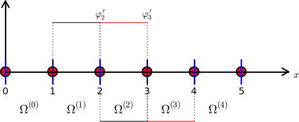
Cellwise computations; assembly

4 P1 elements:

vertices = [0, 0.5, 1, 1.5, 2]
cells = [[0, 1], [1, 2], [2, 3], [3, 4]]
dof_map = [[0], [0, 1], [1, 2], [2]]       # only 1 dof in elm 0, 3

Python code for the assembly algorithm:

# Ae[e][r,s]: element matrix, be[e][r]: element vector
# A[i,j]: coefficient matrix, b[i]: right-hand side

for e in range(len(Ae)):
    for r in range(Ae[e].shape[0]):
        for s in range(Ae[e].shape[1]):
            A[dof_map[e,r],dof_map[e,s]] += Ae[e][i,j]
        b[dof_map[e,r]] += be[e][i,j]

Result: same linear system as arose from computations in the physical domain

General construction of a boundary function

• Now we address nonzero Dirichlet conditions
• \( B(x) \) is not always easy to construct (i.e., extend to the interior of \( \Omega \)), especially not in 2D and 3D
• With finite element basis functions, \( \basphi_i \), \( B(x) \) can be constructed in a completely general way (!)

Define

• \( \Ifb \): set of indices with nodes where \( u \) is known
• \( U_i \): Dirichlet value of \( u \) at node \( i \), \( i\in\Ifb \)

The general formula for \( B \) is now

 
$$ \begin{equation*} B(x) = \sum_{j\in\Ifb} U_j\basphi_j(x) \end{equation*} $$

Explanation

Suppose we have a Dirichlet condition \( u(\xno{k})=U_k \), \( k\in\Ifb \):

 
$$ u(\xno{k}) = \sum_{j\in\Ifb} U_j\underbrace{\basphi_j(x_k)}_{\neq 0 \hbox{ only for }j=k} + \sum_{j\in\If} c_j\underbrace{\basphi_{\nu(j)}(\xno{k})}_{=0,\ k\not\in\If} = U_k $$

Example with two nonzero Dirichlet values; variational formulation

 
$$ -u''=2, \quad u(0)=C,\ u(L)=D $$

 
$$ \int_0^L u'v'\dx = \int_0^L2v\dx\quad\forall v\in V$$

 
$$ (u',v') = (2,v)\quad\forall v\in V$$

Example with two Dirichlet values; boundary function

 
$$ \begin{equation*} B(x) = \sum_{j\in\Ifb} U_j\basphi_j(x) \end{equation*} $$

Here \( \Ifb = \{0,N_n-1\} \), \( U_0=C \), \( U_{N_n-1}=D \); \( \baspsi_i \) are the internal \( \basphi_i \) functions:

 
$$ \baspsi_i = \basphi_{\nu(i)}, \quad \nu(i)=i+1,\quad i\in\If = \{0,\ldots,N=N_n-3\} $$

 
$$ \begin{align*} u(x) &= \underbrace{C\basphi_0 + D\basphi_{N_n-1}}_{B(x)} + \sum_{j\in\If} c_j\basphi_{j+1}\\ &= C\basphi_0 + D\basphi_{N_n-1} + c_0\basphi_1 + c_1\basphi_2 +\cdots + c_N\basphi_{N_n-2} \end{align*} $$

Example with two Dirichlet values; details

Insert \( u = B + \sum_j c_j\baspsi_j \) in variational formulation:

 
$$ (u',v') = (2,v)\quad\Rightarrow\quad (\sum_jc_j\baspsi_j',\baspsi_i') = (2,\baspsi_i)-(B',\baspsi_i')\quad \forall v\in V$$

 
$$ \begin{align*} A_{i-1,j-1} &= \int_0^L \basphi_i'(x)\basphi_j'(x) \dx\\ b_{i-1} &= \int_0^L (f(x)\basphi_i(x) - B'(x)\basphi_i'(x))\dx,\quad B'(x)=C\basphi_{0}'(x) + D\basphi_{N_n-1}'(x) \end{align*} $$

 
for \( i,j = 1,\ldots,N+1=N_n-2 \).

New boundary terms from \( -\int B'\basphi_i'\dx \): add \( C/h \) to \( b_0 \) and \( D/h \) to \( b_N \)

Example with two Dirichlet values; cellwise computations

• All element matrices are as in the previous example
• New element vector in the first and last cell

From the first cell:

 
$$ \tilde b_0^{(1)} = \int_{-1}^1 \left(f\refphi_1 - C\frac{2}{h}\frac{d\refphi_0}{dX}\frac{2}{h}\frac{d\refphi_1}{dX}\right) \frac{h}{2} \dX = \frac{h}{2} 2\int_{-1}^1 \refphi_1 \dX - C\frac{2}{h}(-\frac{1}{2})\frac{2}{h}\frac{1}{2}\frac{h}{2}\cdot 2 = h + C\frac{1}{h}\tp $$

From the last cell:

 
$$ \tilde b_0^{(N_e)} = \int_{-1}^1 \left(f\refphi_0 - D\frac{2}{h}\frac{d\refphi_1}{dX}\frac{2}{h}\frac{d\refphi_0}{dX}\right) \frac{h}{2} \dX = \frac{h}{2} 2\int_{-1}^1 \refphi_0 \dX - D\frac{2}{h}\frac{1}{2}\frac{2}{h}(-\frac{1}{2})\frac{h}{2}\cdot 2 = h + D\frac{1}{h}\tp $$

Modification of the linear system; ideas

• Method 1: incorporate Dirichlet values through a \( B(x) \) function and demand \( \baspsi_i=0 \) where Dirichlet values apply
• Method 2: drop \( B(x) \), drop demands to \( \baspsi_i \), just assemble as if there were no Dirichlet conditions, and modify the linear system instead

Method 2: always choose \( \baspsi_i = \basphi_i \) for all \( i\in\If \) and set

 
$$ \begin{equation*} u(x) = \sum_{j\in\If}c_j\basphi_j(x),\quad \If=\{0,\ldots,N=N_n-1\} \end{equation*} $$

Modification of the linear system; original system

 
$$ -u''=2,\quad u(0)=0,\ u(L)=D$$

Assemble as if there were no Dirichlet conditions:

 
$$ \begin{equation*} { \frac{1}{h}\left( \begin{array}{ccccccccc} 1 & -1 & 0 &\cdots & \cdots & \cdots & \cdots & \cdots & 0 \\ -1 & 2 & -1 & \ddots & & & & & \vdots \\ 0 & -1 & 2 & -1 & \ddots & & & & \vdots \\ \vdots & \ddots & & \ddots & \ddots & 0 & & & \vdots \\ \vdots & & \ddots & \ddots & \ddots & \ddots & \ddots & & \vdots \\ \vdots & & & 0 & -1 & 2 & -1 & \ddots & \vdots \\ \vdots & & & & \ddots & \ddots & \ddots &\ddots & 0 \\ \vdots & & & & &\ddots & \ddots &\ddots & -1 \\ 0 &\cdots & \cdots &\cdots & \cdots & \cdots & 0 & -1 & 1 \end{array} \right) \left( \begin{array}{c} c_0 \\ \vdots\\ \vdots\\ \vdots \\ \vdots \\ \vdots \\ \vdots \\ \vdots\\ c_{N} \end{array} \right) = \left( \begin{array}{c} h \\ 2h\\ \vdots\\ \vdots \\ \vdots \\ \vdots \\ \vdots \\ 2h\\ h \end{array} \right) } \end{equation*} $$

Modification of the linear system; row replacement

• Dirichlet condition \( u(\xno{k})= U_k \) means \( c_k=U_k \)
  (since \( c_k=u(\xno{k}) \))
• Replace first row by \( c_0=0 \)
• Replace last row by \( c_N=D \)

 
$$ \begin{equation*} { \frac{1}{h}\left( \begin{array}{ccccccccc} h & 0 & 0 &\cdots & \cdots & \cdots & \cdots & \cdots & 0 \\ -1 & 2 & -1 & \ddots & & & & & \vdots \\ 0 & -1 & 2 & -1 & \ddots & & & & \vdots \\ \vdots & \ddots & & \ddots & \ddots & 0 & & & \vdots \\ \vdots & & \ddots & \ddots & \ddots & \ddots & \ddots & & \vdots \\ \vdots & & & 0 & -1 & 2 & -1 & \ddots & \vdots \\ \vdots & & & & \ddots & \ddots & \ddots &\ddots & 0 \\ \vdots & & & & &\ddots & \ddots &\ddots & -1 \\ 0 &\cdots & \cdots &\cdots & \cdots & \cdots & 0 & 0 & h \end{array} \right) \left( \begin{array}{c} c_0 \\ \vdots\\ \vdots\\ \vdots \\ \vdots \\ \vdots \\ \vdots \\ \vdots\\ c_{N} \end{array} \right) = \left( \begin{array}{c} 0 \\ 2h\\ \vdots\\ \vdots \\ \vdots \\ \vdots \\ \vdots \\ 2h\\ D \end{array} \right) } \end{equation*} $$

Modification of the linear system; element matrix/vector

In cell 0 we know \( u \) for local node (degree of freedom) \( r=0 \). Replace the first cell equation by \( \tilde c_0 = 0 \):

 
$$ \begin{equation*} \tilde A^{(0)} = A = \frac{1}{h}\left(\begin{array}{rr} h & 0\\ -1 & 1 \end{array}\right),\quad \tilde b^{(0)} = \left(\begin{array}{c} 0\\ h \end{array}\right) \end{equation*} $$

In cell \( N_e \) we know \( u \) for local node \( r=1 \). Replace the last equation in the cell system by \( \tilde c_1=D \):

 
$$ \begin{equation*} \tilde A^{(N_e)} = A = \frac{1}{h}\left(\begin{array}{rr} 1 & -1\\ 0 & h \end{array}\right),\quad \tilde b^{(N_e)} = \left(\begin{array}{c} h\\ D \end{array}\right) \end{equation*} $$

Symmetric modification of the linear system; algorithm

• The modification above destroys symmetry of the matrix: e.g., \( A_{0,1}\neq A_{1,0} \)
• Symmetry is often important in 2D and 3D
  (faster computations, less storage)
• A more complex modification can preserve symmetry!

Algorithm for incorporating \( c_i=U_i \) in a symmetric way:

1. Subtract column \( i \) times \( U_i \) from the right-hand side
2. Zero out column and row no \( i \)
3. Place 1 on the diagonal
4. Set \( b_i=U_i \)

Symmetric modification of the linear system; example

 
$$ \begin{equation*} { \frac{1}{h}\left( \begin{array}{ccccccccc} h & 0 & 0 &\cdots & \cdots & \cdots & \cdots & \cdots & 0 \\ 0 & 2 & -1 & \ddots & & & & & \vdots \\ 0 & -1 & 2 & -1 & \ddots & & & & \vdots \\ \vdots & \ddots & & \ddots & \ddots & 0 & & & \vdots \\ \vdots & & \ddots & \ddots & \ddots & \ddots & \ddots & & \vdots \\ \vdots & & & 0 & -1 & 2 & -1 & \ddots & \vdots \\ \vdots & & & & \ddots & \ddots & \ddots &\ddots & 0 \\ \vdots & & & & &\ddots & \ddots &\ddots & 0 \\ 0 &\cdots & \cdots &\cdots & \cdots & \cdots & 0 & 0 & h \end{array} \right) \left( \begin{array}{c} c_0 \\ \vdots\\ \vdots\\ \vdots \\ \vdots \\ \vdots \\ \vdots \\ \vdots\\ c_{N} \end{array} \right) = \left( \begin{array}{c} 0 \\ 2h\\ \vdots\\ \vdots \\ \vdots \\ \vdots \\ \vdots \\ 2h +\frac{D}{h}\\ D \end{array} \right) } \end{equation*} $$

Symmetric modification of the linear system; element level

Symmetric modification applied to \( \tilde A^{(N_e)} \):

 
$$ \begin{equation*} \tilde A^{(N_e)} = A = \frac{1}{h}\left(\begin{array}{rr} 1 & 0\\ 0 & h \end{array}\right),\quad \tilde b^{(N_e)} = \left(\begin{array}{c} h + D/h\\ D \end{array}\right) \end{equation*} $$

Boundary conditions: specified derivative

 
$$ -u''=f,\quad u'(0)=C,\ u(L)=D$$

• \( \baspsi_i(L)=0 \) because of Dirichlet condition \( u(L)=D \)
  (or no demand and modify linear system)
• No demand to \( \baspsi_i(0) \)
• The condition \( u'(0)=C \) will be handled (as usual) through a boundary term arising from integration by parts

The variational formulation

Galerkin's method:

 
$$ \begin{equation*} \int_0^L(u''(x)+f(x))\baspsi_i(x) dx = 0,\quad i\in\If \end{equation*} $$

Integration of \( u''\baspsi_i \) by parts:

 
$$ \begin{equation*} \int_0^Lu'(x)\baspsi_i'(x) \dx -(u'(L)\baspsi_i(L) - u'(0)\baspsi_i(0)) - \int_0^L f(x)\baspsi_i(x) \dx =0 \end{equation*} $$

• \( u'(L){\baspsi_i(L)}=0 \) since \( \baspsi_i(L)=0 \)
• \( u'(0)\baspsi_i(0) = C\baspsi_i(0) \) since \( u'(0)=C \)

Method 1: Boundary function and exclusion of Dirichlet degrees of freedom

• \( \baspsi_i = \basphi_i \), \( i\in\If =\{0,\ldots,N=N_n-2\} \)
• \( B(x)=D\basphi_{N_n-1}(x) \), \( u= B + \sum_{j=0}^N c_j\basphi_j \)

 
$$ \begin{equation*} \int_0^Lu'(x)\basphi_i'(x) dx = \int_0^L f(x)\basphi_i(x) dx - C\basphi_i(0),\quad i\in\If \end{equation*} $$

 
$$ \begin{equation*} \sum_{j=0}^{N}\left( \int_0^L \basphi_i'\basphi_j' dx \right)c_j = \int_0^L\left(f\basphi_i -D\basphi_N'\basphi_i\right) dx - C\basphi_i(0) \end{equation*} $$

 
for \( i=0,\ldots,N=N_n-2 \).

Method 2: Use all \( \basphi_i \) and insert the Dirichlet condition in the linear system

• Now \( \baspsi_i=\basphi_i \), \( i=0,\ldots,N=N_n-1 \) (all nodes)
• \( \basphi_N(L)\neq 0 \), so \( u'(L)\basphi_N(L)\neq 0 \)
• However, the term \( u'(L)\basphi_N(L) \) in \( b_N \) will be erased when we insert the Dirichlet value in \( b_N=D \)

We can therefore forget about the term \( u'(L)\basphi_i(L) \)!

 
$$ \begin{equation*} u(x) = \sum_{j=0}^{N=N_n-1} c_j\basphi_j(x) \end{equation*} $$

 
$$ \begin{equation*} \sum_{j=0}^{N=N_n-1}\left( \int_0^L \basphi_i'(x)\basphi_j'(x) dx \right)c_j = \int_0^L f(x)\basphi_i(x) dx - C\basphi_i(0) \end{equation*} $$

Assemble entries for \( i=0,\ldots,N=N_n-1 \) and then modify the last equation to \( c_N=D \)

How the Neumann condition impacts the element matrix and vector

The extra term \( C\basphi_0(0) \) affects only the element vector from the first cell since \( \basphi_0=0 \) on all other cells.

 
$$ \begin{equation*} \tilde A^{(0)} = A = \frac{1}{h}\left(\begin{array}{rr} 1 & 1\\ -1 & 1 \end{array}\right),\quad \tilde b^{(0)} = \left(\begin{array}{c} h - C\\ h \end{array}\right) \end{equation*} $$

The finite element algorithm

The differential equation problem defines the integrals in the variational formulation.

Request these functions from the user:

integrand_lhs(phi, r, s, x)
boundary_lhs(phi, r, s, x)
integrand_rhs(phi, r, x)
boundary_rhs(phi, r, x)

Must also have a mesh with vertices, cells, and dof_map

Python pseudo code; the element matrix and vector

<Declare global matrix, global rhs: A, b>

# Loop over all cells
for e in range(len(cells)):

    # Compute element matrix and vector
    n = len(dof_map[e])  # no of dofs in this element
    h = vertices[cells[e][1]] - vertices[cells[e][0]]
    <Declare element matrix, element vector: A_e, b_e>

    # Integrate over the reference cell
    points, weights = <numerical integration rule>
    for X, w in zip(points, weights):
        phi = <basis functions + derivatives at X>
        detJ = h/2
        x = <affine mapping from X>
        for r in range(n):
            for s in range(n):
                A_e[r,s] += integrand_lhs(phi, r, s, x)*detJ*w
            b_e[r] += integrand_rhs(phi, r, x)*detJ*w

    # Add boundary terms
    for r in range(n):
        for s in range(n):
            A_e[r,s] += boundary_lhs(phi, r, s, x)*detJ*w
        b_e[r] += boundary_rhs(phi, r, x)*detJ*w

Python pseudo code; boundary conditions and assembly

for e in range(len(cells)):
    ...

    # Incorporate essential boundary conditions
    for r in range(n):
        global_dof = dof_map[e][r]
        if global_dof in essbc_dofs:
            # dof r is subject to an essential condition
            value = essbc_docs[global_dof]
            # Symmetric modification
            b_e -= value*A_e[:,r]
            A_e[r,:] = 0
            A_e[:,r] = 0
            A_e[r,r] = 1
            b_e[r] = value

    # Assemble
    for r in range(n):
        for s in range(n):
            A[dof_map[e][r], dof_map[e][r]] += A_e[r,s]
        b[dof_map[e][r] += b_e[r]

<solve linear system>

Variational formulations in 2D and 3D

Integration by parts

• \( \partial\Omega_N \): Neumann conditions \( -a\frac{\partial u}{\partial n} = g \)
• \( \partial\Omega_D \): Dirichlet conditions \( u = u_0 \)
• \( v\in V \) must vanish on \( \partial\Omega_D \) (in method 1)

Example on integration by parts; problem

 
$$ \begin{align*} \v\cdot\nabla u + \beta u &= \nabla\cdot\left( \dfc\nabla u\right) + f, \quad & \x\in\Omega\\ u &= u_0,\quad &\x\in\partial\Omega_D\\ -\dfc\frac{\partial u}{\partial n} &= g,\quad &\x\in\partial\Omega_N \end{align*} $$

• Known: \( \dfc \), \( \beta \), \( f \), \( u_0 \), and \( g \).
• Second-order PDE: must have exactly one boundary condition at each point of the boundary

Method 1 with boundary function and \( \baspsi_i=0 \) on \( \partial\Omega_D \) (ensures \( u=u_0 \) condition):

 
$$ u(\x) = B(\x) + \sum_{j\in\If} c_j\baspsi_j(\x),\quad B(\x)=u_0(\x) $$

Example on integration by parts in 1D/2D/3D

Galerkin's method: multiply by \( v\in V \) and integrate over \( \Omega \),

 
$$ \int_{\Omega} (\v\cdot\nabla u + \beta u)v\dx = \int_{\Omega} \nabla\cdot\left( \dfc\nabla u\right)v\dx + \int_{\Omega}fv \dx $$

Integrate the second-order term by parts according to the formula:

 
$$ \int_{\Omega} \nabla\cdot\left( \dfc\nabla u\right) v \dx = -\int_{\Omega} \dfc\nabla u\cdot\nabla v\dx + \int_{\partial\Omega} \dfc\frac{\partial u}{\partial n} v\ds, $$

Galerkin's method then gives

 
$$ \int_{\Omega} (\v\cdot\nabla u + \beta u)v\dx = -\int_{\Omega} \dfc\nabla u\cdot\nabla v\dx + \int_{\partial\Omega} \dfc\frac{\partial u}{\partial n} v\ds + \int_{\Omega} fv \dx $$

Incorporation of the Neumann condition in the variational formulation

Note: \( v\neq 0 \) only on \( \partial\Omega_N \) (since \( v=0 \) on \( \partial\Omega_D \)):

 
$$ \int_{\partial\Omega} \dfc\frac{\partial u}{\partial n} v\ds = \int_{\partial\Omega_N} \underbrace{\dfc\frac{\partial u}{\partial n}}_{-g} v\ds = -\int_{\partial\Omega_N} gv\ds $$

The final variational form:

 
$$ \int_{\Omega} (\v\cdot\nabla u + \beta u)v\dx = -\int_{\Omega} \dfc\nabla u\cdot\nabla v \dx - \int_{\partial\Omega_N} g v\ds + \int_{\Omega} fv \dx $$

Or with inner product notation:

 
$$ (\v\cdot\nabla u, v) + (\beta u,v) = - (\dfc\nabla u,\nabla v) - (g,v)_{N} + (f,v) $$

\( (g,v)_{N} \): line or surface integral over \( \partial\Omega_N \).

Derivation of the linear system

• \( \forall v\in V \) is replaced by for all \( \baspsi_i \), \( i\in\If \)
• Insert \( u = B + \sum_{j\in\If} c_j\baspsi_j \), \( B = u_0 \), in the variational form
• Identify \( i,j \) terms (matrix) and \( i \) terms (right-hand side)
• Write on form \( \sum_{i\in\If}A_{i,j}c_j = b_i \), \( i\in\If \)

 
$$ A_{i,j} = (\v\cdot\nabla \baspsi_j, \baspsi_i) + (\beta \baspsi_j ,\baspsi_i) + (\dfc\nabla \baspsi_j,\nabla \baspsi_i) $$

 
$$ b_i = (g,\baspsi_i)_{N} + (f,\baspsi_i) - (\v\cdot\nabla u_0, \baspsi_i) + (\beta u_0 ,\baspsi_i) + (\dfc\nabla u_0,\nabla \baspsi_i) $$

Transformation to a reference cell in 2D/3D (1)

 
$$ \begin{equation*} \int_{{\Omega}^{(e)}} \dfc(\x)\nabla\basphi_i\cdot\nabla\basphi_j\dx \end{equation*} $$

Mapping from reference to physical coordinates:

 
$$ \x(\X) $$

with Jacobian \( J \),

 
$$ J_{i,j}=\frac{\partial x_j}{\partial X_i} $$

Transformation to a reference cell in 2D/3D (2)

• \( \dx \rightarrow \det J\dX \).
• Must express \( \nabla\basphi_i \) by an expression with \( \refphi_r \), \( i=q(e,r) \): \( \nabla\refphi_r(\X) \)
• We want \( \nabla_{\x}\refphi_r(\X) \) (derivatives wrt \( \x \))
• What we readily have is \( \nabla_{\X}\refphi_r(\X) \) (derivative wrt \( \X \))
• Need to transform \( \nabla_{\X}\refphi_r(\X) \) to \( \nabla_{\x}\refphi_r(\X) \)

Transformation to a reference cell in 2D/3D (3)

Can derive

 
$$ \begin{align*} \nabla_{\X}\refphi_r &= J\cdot\nabla_{\x}\basphi_i\\ \nabla_{\x}\basphi_i &= \nabla_{\x}\refphi_r(\X) = J^{-1}\cdot\nabla_{\X}\refphi_r(\X) \end{align*} $$

Integral transformation from physical to reference coordinates:

 
$$ \begin{equation*} \int_{\Omega^{(e)}} \dfc(\x)\nabla_{\x}\basphi_i\cdot\nabla_{\x}\basphi_j\dx = \int_{\tilde\Omega^r} \dfc(\x(\X))(J^{-1}\cdot\nabla_{\X}\refphi_r)\cdot (J^{-1}\cdot\nabla\refphi_s)\det J\dX \end{equation*} $$

Numerical integration

Numerical integration over reference cell triangles and tetrahedra:

 
$$ \int_{\tilde\Omega^r} g\dX = \sum_{j=0}^{n-1} w_j g(\bar\X_j)$$

Module numint.py contains different rules:

>>> import numint
>>> x, w = numint.quadrature_for_triangles(num_points=3)
>>> x
[(0.16666666666666666, 0.16666666666666666),
 (0.66666666666666666, 0.16666666666666666),
 (0.16666666666666666, 0.66666666666666666)]
>>> w
[0.16666666666666666, 0.16666666666666666, 0.16666666666666666]

• Triangle: rules with \( n=1,3,4,7 \) integrate exactly polynomials of degree \( 1,2,3,4 \), resp.
• Tetrahedron: rules with \( n=1,4,5,11 \) integrate exactly polynomials of degree \( 1,2,3,4 \), resp.