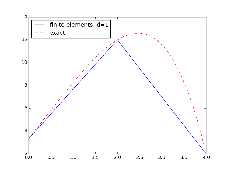
Figure 3: Finite element and exact solution using two cells.
At this point, it is sensible to create a program with symbolic calculations to perform all the steps in the computational machinery, both for automating the work and for documenting the complete algorithms. As we have seen, there are quite many details involved with finite element computations and incorporation of boundary conditions. An implementation will also act as a structured summary of all these details.
We first consider implementations when \( \baspsi_i \) are global functions are hence different from zero on most of \( \Omega =[0,L] \) so all integrals need integration over the entire domain. (Finite element basis functions, where we utilize their local support and perform integrations over cells, will be treated later.) Since the expressions for the entries in the linear system depend on the differential equation problem being solved, the user must supply the necessary formulas via Python functions. The implementations here attempt to perform symbolic calculations, but fall back on numerical computations if the symbolic ones fail.
The user must prepare a function
integrand_lhs(psi, i, j) for returning the integrand of the
integral that contributes to matrix entry \( (i,j) \).
The psi variable is a Python dictionary holding the basis
functions and their derivatives in symbolic form. More precisely,
psi[q] is a list of
$$
\begin{equation*}
\{\frac{d^q\baspsi_0}{dx^q},\ldots,\frac{d^q\baspsi_{N_n-1}}{dx^q}\}
\tp
\end{equation*}
$$
Similarly, integrand_rhs(psi, i) returns the integrand
for entry number \( i \) in the right-hand side vector.
Since we also have contributions to the right-hand side vector
(and potentially also the
matrix) from boundary terms without any integral, we introduce two
additional functions, boundary_lhs(psi, i, j) and
boundary_rhs(psi, i) for returning terms in the variational
formulation that are not to be integrated over the domain \( \Omega \).
Examples, to be shown later, will explain in more detail how these
user-supplied function may look like.
The linear system can be computed and solved symbolically by the following function:
import sympy as sym

def solver(integrand_lhs, integrand_rhs, psi, Omega,
           boundary_lhs=None, boundary_rhs=None):
    N = len(psi[0]) - 1
    A = sym.zeros((N+1, N+1))
    b = sym.zeros((N+1, 1))
    x = sym.Symbol('x')
    for i in range(N+1):
        for j in range(i, N+1):
            integrand = integrand_lhs(psi, i, j)
            I = sym.integrate(integrand, (x, Omega[0], Omega[1]))
            if boundary_lhs is not None:
                I += boundary_lhs(psi, i, j)
            A[i,j] = A[j,i] = I   # assume symmetry
        integrand = integrand_rhs(psi, i)
        I = sym.integrate(integrand, (x, Omega[0], Omega[1]))
        if boundary_rhs is not None:
            I += boundary_rhs(psi, i)
        b[i,0] = I
    c = A.LUsolve(b)
    u = sum(c[i,0]*psi[0][i] for i in range(len(psi[0])))
    return u, c
Not surprisingly, symbolic solution of differential
equations, discretized by a Galerkin or least squares method
with global basis functions,
is of limited interest beyond the simplest problems, because
symbolic integration might be very time consuming or impossible, not
only in sympy but also in
WolframAlpha
(which applies the perhaps most powerful symbolic integration
software available today: Mathematica). Numerical integration
as an option is therefore desirable.
The extended solver function below tries to combine symbolic and
numerical integration. The latter can be enforced by the user, or it
can be invoked after a non-successful symbolic integration (being
detected by an Integral object as the result of the integration
in sympy).
Note that for a
numerical integration, symbolic expressions must be converted to
Python functions (using lambdify), and the expressions cannot contain
other symbols than x. The real solver routine in the
varform1D.py
file has error checking and meaningful error messages in such cases.
The solver code below is a condensed version of the real one, with
the purpose of showing how to automate the Galerkin or least squares
method for solving differential equations in 1D with global basis functions:
def solver(integrand_lhs, integrand_rhs, psi, Omega,
           boundary_lhs=None, boundary_rhs=None, symbolic=True):
    N = len(psi[0]) - 1
    A = sym.zeros((N+1, N+1))
    b = sym.zeros((N+1, 1))
    x = sym.Symbol('x')
    for i in range(N+1):
        for j in range(i, N+1):
            integrand = integrand_lhs(psi, i, j)
            if symbolic:
                I = sym.integrate(integrand, (x, Omega[0], Omega[1]))
                if isinstance(I, sym.Integral):
                    symbolic = False  # force num.int. hereafter
            if not symbolic:
                integrand = sym.lambdify([x], integrand)
                I = sym.mpmath.quad(integrand, [Omega[0], Omega[1]])
            if boundary_lhs is not None:
                I += boundary_lhs(psi, i, j)
            A[i,j] = A[j,i] = I
        integrand = integrand_rhs(psi, i)
        if symbolic:
            I = sym.integrate(integrand, (x, Omega[0], Omega[1]))
            if isinstance(I, sym.Integral):
                symbolic = False
        if not symbolic:
            integrand = sym.lambdify([x], integrand)
            I = sym.mpmath.quad(integrand, [Omega[0], Omega[1]])
        if boundary_rhs is not None:
            I += boundary_rhs(psi, i)
        b[i,0] = I
    c = A.LUsolve(b)
    u = sum(c[i,0]*psi[0][i] for i in range(len(psi[0])))
    return u, c
To demonstrate the code above, we address $$ \begin{equation*} -u''(x)=b,\quad x\in\Omega=[0,1],\quad u(0)=1,\ u(1)=0,\end{equation*} $$ with \( b \) as a (symbolic) constant. A possible basis for the space \( V \) is \( \baspsi_i(x) = x^{i+1}(1-x) \), \( i\in\If \). Note that \( \baspsi_i(0)=\baspsi_i(1)=0 \) as required by the Dirichlet conditions. We need a \( B(x) \) function to take care of the known boundary values of \( u \). Any function \( B(x)=1-x^p \), \( p\in\Real \), is a candidate, and one arbitrary choice from this family is \( B(x)=1-x^3 \). The unknown function is then written as $$ \begin{equation*} u(x) = B(x) + \sum_{j\in\If} c_j\baspsi_j(x)\tp \end{equation*} $$
Let us use the Galerkin method to derive the variational formulation. Multiplying the differential equation by \( v \) and integrating by parts yield $$ \begin{equation*} \int_0^1 u'v' \dx = \int_0^1 fv \dx\quad\forall v\in V, \end{equation*} $$ and with \( u=B + \sum_jc_j\baspsi_j \) we get the linear system $$ \begin{equation} \sum_{j\in\If}\left(\int_0^1\baspsi_i'\baspsi_j' \dx\right)c_j = \int_0^1(f\baspsi_i-B'\baspsi_i') \dx, \quad i\in\If\tp \tag{81} \end{equation} $$
The application can be coded as follows with sympy:
import sympy as sym
x, b = sym.symbols('x b')
f = b
B = 1 - x**3
dBdx = sym.diff(B, x)

# Compute basis functions and their derivatives
N = 3
psi = {0: [x**(i+1)*(1-x) for i in range(N+1)]}
psi[1] = [sym.diff(psi_i, x) for psi_i in psi[0]]

def integrand_lhs(psi, i, j):
    return psi[1][i]*psi[1][j]

def integrand_rhs(psi, i):
    return f*psi[0][i] - dBdx*psi[1][i]

Omega = [0, 1]

from varform1D import solver
u_bar, c = solver(integrand_lhs, integrand_rhs, psi, Omega,
                  verbose=True, symbolic=True)
u = B + u_bar
print 'solution u:', sym.simplify(sym.expand(u))
The printout of u reads -b*x**2/2 + b*x/2 - x + 1.
Note that expanding u, before simplifying, is necessary
in the present case
to get a compact, final expression with sympy. Doing expand before
simplify is a common strategy for simplifying expressions in
sympy. However,
a non-expanded u might be preferable in other cases - this depends on
the problem in question.
The exact solution \( \uex(x) \) can be derived by
some sympy code that closely follows the examples in
the section Simple model problems and their solutions. The idea is to integrate
\( -u''=b \) twice and determine the integration constants from
the boundary conditions:
C1, C2 = sym.symbols('C1 C2')    # integration constants
f1 = sym.integrate(f, x) + C1
f2 = sym.integrate(f1, x) + C2
# Find C1 and C2 from the boundary conditions u(0)=0, u(1)=1
s = sym.solve([u_e.subs(x,0) - 1, u_e.subs(x,1) - 0], [C1, C2])
# Form the exact solution
u_e = -f2 + s[C1]*x + s[C2]
print 'analytical solution:', u_e
print 'error:', sym.simplify(sym.expand(u - u_e))
The last line prints 0, which is not surprising when
\( \uex(x) \) is a parabola and our approximate \( u \) contains polynomials up to
degree 4. It suffices to have \( N=1 \), i.e., polynomials of degree
2, to recover the exact solution.
We can play around with the code and test that with \( f=Kx^p \), for some constants \( K \) and \( p \), the solution is a polynomial of degree \( p+2 \), and \( N=p+1 \) guarantees that the approximate solution is exact.
Although the symbolic code is capable of integrating many choices of \( f(x) \), the symbolic expressions for \( u \) quickly become lengthy and non-informative, so numerical integration in the code, and hence numerical answers, have the greatest application potential.
Implementation of the finite element algorithms for differential equations follows closely the algorithm for approximation of functions. The new additional ingredients are
ilhs(e, phi, r, s, X, x, h)irhs(e, phi, r, X, x, h)blhs (e, phi, r, s, X, x, h)brhs (e, phi, r, s, X, x, h)phi is a dictionary where phi[q] holds a list of the
derivatives of order q of the basis functions with respect to the
physical coordinate \( x \). The derivatives are available as Python
functions of X. For example, phi[0][r](X) means \( \refphi_r(X) \),
and phi[1][s](X, h) means \( d\refphi_s (X)/dx \) (we refer to
the file fe1D.py for details
regarding the function basis that computes the phi
dictionary). The r and s
arguments in the above functions correspond to the index in the
integrand contribution from an integration point to \( \tilde
A^{(e)}_{r,s} \) and \( \tilde b^{(e)}_r \). The variables e and h are
the current element number and the length of the cell, respectively.
Specific examples below will make it clear how to construction these
Python functions.
Given a mesh represented by vertices, cells, and dof_map as
explained before, we can write a pseudo Python code to list all
the steps in the computational algorithm for finite element solution
of a differential equation.
<Declare global matrix and rhs: A, b>

for e in range(len(cells)):

    # Compute element matrix and vector
    n = len(dof_map[e])  # no of dofs in this element
    h = vertices[cells[e][1]] - vertices[cells[e][1]]
    <Initialize element matrix and vector: A_e, b_e>

    # Integrate over the reference cell
    points, weights = <numerical integration rule>
    for X, w in zip(points, weights):
        phi = <basis functions and derivatives at X>
        detJ = h/2
        dX = detJ*w

        x = <affine mapping from X>
        for r in range(n):
            for s in range(n):
                A_e[r,s] += ilhs(e, phi, r, s, X, x, h)*dX
            b_e[r] += irhs(e, phi, r, X, x, h)*dX

    # Add boundary terms
    for r in range(n):
        for s in range(n):
            A_e[r,s] += blhs(e, phi, r, s, X, x)*dX
        b_e[r] += brhs(e, phi, r, X, x, h)*dX

    # Incorporate essential boundary conditions
    for r in range(n):
        global_dof = dof_map[e][r]
        if global_dof in essbc:
            # local dof r is subject to an essential condition
            value = essbc[global_dof]
            # Symmetric modification
            b_e -= value*A_e[:,r]
            A_e[r,:] = 0
            A_e[:,r] = 0
            A_e[r,r] = 1
            b_e[r] = value

    # Assemble
    for r in range(n):
        for s in range(n):
            A[dof_map[e][r], dof_map[e][s]] += A_e[r,s]
        b[dof_map[e][r] += b_e[r]

<solve linear system>
A complete function finite_element1D_naive
for the 1D finite algorithm above, is found in the file
fe1D.py. The term "naive" refers
to a version of the algorithm where we use a standard dense square matrix
as global matrix A. The implementation also has a verbose mode for
printing out the element matrices and vectors as they are computed.
Below is the complete function without the print statements.
def finite_element1D_naive(
    vertices, cells, dof_map,     # mesh
    essbc,                        # essbc[globdof]=value
    ilhs,                         # integrand left-hand side
    irhs,                         # integrand right-hand side
    blhs=lambda e, phi, r, s, X, x, h: 0,
    brhs=lambda e, phi, r, X, x, h: 0,
    intrule='GaussLegendre',      # integration rule class
    verbose=False,                # print intermediate results?
    ):
    N_e = len(cells)
    N_n = np.array(dof_map).max() + 1

    A = np.zeros((N_n, N_n))
    b = np.zeros(N_n)

    for e in range(N_e):
        Omega_e = [vertices[cells[e][0]], vertices[cells[e][1]]]
        h = Omega_e[1] - Omega_e[0]

        d = len(dof_map[e]) - 1  # Polynomial degree
        # Compute all element basis functions and their derivatives
        phi = basis(d)

        # Element matrix and vector
        n = d+1  # No of dofs per element
        A_e = np.zeros((n, n))
        b_e = np.zeros(n)

        # Integrate over the reference cell
        if intrule == 'GaussLegendre':
            points, weights = GaussLegendre(d+1)
        elif intrule == 'NewtonCotes':
            points, weights = NewtonCotes(d+1)

        for X, w in zip(points, weights):
            detJ = h/2
            x = affine_mapping(X, Omega_e)
            dX = detJ*w

            # Compute contribution to element matrix and vector
            for r in range(n):
                for s in range(n):
                    A_e[r,s] += ilhs(phi, r, s, X, x, h)*dX
                b_e[r] += irhs(phi, r, X, x, h)*dX

        # Add boundary terms
        for r in range(n):
            for s in range(n):
                A_e[r,s] += blhs(phi, r, s, X, x, h)
            b_e[r] += brhs(phi, r, X, x, h)

        # Incorporate essential boundary conditions
        modified = False
        for r in range(n):
            global_dof = dof_map[e][r]
            if global_dof in essbc:
                # dof r is subject to an essential condition
                value = essbc[global_dof]
                # Symmetric modification
                b_e -= value*A_e[:,r]
                A_e[r,:] = 0
                A_e[:,r] = 0
                A_e[r,r] = 1
                b_e[r] = value
                modified = True

        # Assemble
        for r in range(n):
            for s in range(n):
                A[dof_map[e][r], dof_map[e][s]] += A_e[r,s]
            b[dof_map[e][r]] += b_e[r]

    c = np.linalg.solve(A, b)
    return c, A, b, timing
The timing object is a dictionary holding the CPU spent on computing
A and the CPU time spent on solving the linear system. (We have
left out the timing statements.)
A potential efficiency problem with the finite_element1D_naive function
is that it uses dense \( (N+1)\times (N+1) \) matrices, while we know that
only \( 2d+1 \) diagonals around the main diagonal are different from zero.
Switching to a sparse matrix is very easy. Using the DOK (dictionary of
keys) format, we declare A as
import scipy.sparse
A = scipy.sparse.dok_matrix((N_n, N_n))
Assignments or in-place arithmetics are done as for a dense matrix,
A[i,j] += term
A[i,j]  = term
but only the index pairs (i,j) we have used in assignments or
in-place arithmetics are actually stored.
A tailored solution algorithm is needed. The most reliable is
sparse Gaussian elimination:
import scipy.sparse.linalg
c = scipy.sparse.linalg.spsolve(A.tocsr(), b, use_umfpack=True)
The declaration of A and the solve statement are the only
changes needed in the finite_element1D_naive to utilize
sparse matrices. The resulting modification is found in the
function finite_element1D.
Let us demonstrate the finite element software on
$$ -u''(x)=f(x),\quad x\in (0,L),\quad u'(0)=C,\ u(L)=D\tp$$
This problem can be analytically solved by the
model2 function from the section Simple model problems and their solutions.
Let \( f(x)=x^2 \). Calling model2(x**2, L, C, D) gives
$$ u(x) = D + C(x-L) + \frac{1}{12}(L^4 - x^4) $$
The variational formulation reads
$$ (u', v) = (x^2, v) - Cv(0)\tp$$
The entries in the element matrix and vector,
which we need to set up the ilhs, irhs,
blhs, and brhs functions, becomes
$$
\begin{align*}
A^{(e)}_{r,s} &= \int_{-1}^1 \frac{d\refphi_r}{dx}\frac{\refphi_s}{dx}(\det J\dX),\\
b^{(e)} &= \int_{-1}^1 x^2\refphi_r\det J\dX - C\refphi_r(-1)I(e,0),
\end{align*}
$$
where \( I(e) \) is an indicator function: \( I(e,q)=1 \) if \( e=q \), otherwise \( I(e)=0 \).
We use this indicator function to formulate that the boundary term
\( Cv(0) \), which in the local element coordinate system becomes \( C\refphi_r(-1) \),
is only included for the element \( e=0 \).
The functions for specifying the element matrix and vector entries
must contain the integrand, but without the \( \det J\dX \) term, and
the derivatives \( d\refphi_r(X)/dx \)
with respect to the physical \( x \) coordinates are
contained in phi[1][r](X), computed by the function basis.
def ilhs(e, phi, r, s, X, x, h):
    return phi[1][r](X, h)*phi[1][s](X, h)

def irhs(e, phi, r, X, x, h):
    return x**2*phi[0][r](X)

def blhs(e, phi, r, s, X, x, h):
    return 0

def brhs(e, phi, r, X, x, h):
    return -C*phi[0][r](-1) if e == 0 else 0
We can then make the call to finite_element1D_naive or finite_element1D
to solve the problem with two P1 elements:
from fe1D import finite_element1D_naive, mesh_uniform
C = 5;  D = 2;  L = 4
d = 1

vertices, cells, dof_map = mesh_uniform(
    N_e=2, d=d, Omega=[0,L], symbolic=False)
essbc = {}
essbc[dof_map[-1][-1]] = D

c, A, b, timing = finite_element1D(
    vertices, cells, dof_map, essbc,
    ilhs=ilhs, irhs=irhs, blhs=blhs, brhs=brhs,
    intrule='GaussLegendre')
It remains to plot the solution (with high resolution in each element).
To this end, we use the u_glob function imported from
fe1D, which imports it from fe_approx1D_numit (the
u_glob function in fe_approx1D.py
works with elements and nodes, while u_glob in
fe_approx1D_numint works with cells, vertices,
and dof_map):
u_exact = lambda x: D + C*(x-L) + (1./6)*(L**3 - x**3)
from fe1D import u_glob
x, u, nodes = u_glob(c, cells, vertices, dof_map)
u_e = u_exact(x, C, D, L)
print u_exact(nodes, C, D, L) - c  # difference at the nodes

import matplotlib.pyplot as plt
plt.plot(x, u, 'b-', x, u_e, 'r--')
plt.legend(['finite elements, d=%d' %d, 'exact'], loc='upper left')
plt.show()
The result is shown in Figure 3. We see that the solution using P1 elements is exact at the nodes, but feature considerable discrepancy between the nodes. Exercise 10: Investigate exact finite element solutions asks you to explore this problem further using other \( m \) and \( d \) values.
Figure 3: Finite element and exact solution using two cells.