Figure 2: Illustration of the derivative of piecewise linear basis functions associated with nodes in cell 2.
The purpose of this section is to demonstrate in detail how the finite element method can the be applied to the model problem $$ -u''(x) = 2,\quad x\in (0,L),\ u(0)=u(L)=0,$$ with variational formulation $$ (u',v') = (2,v)\quad\forall v\in V\tp $$ Any \( v\in V \) must obey \( v(0)=v(L)=0 \) because of the Dirichlet conditions on \( u \). The variational formulation is derived in the section Integration by parts.
We introduce a finite element mesh with \( N_e \) cells, all with length \( h \), and number the cells from left to right. Choosing P1 elements, there are two nodes per cell, and the coordinates of the nodes become $$ \begin{equation*} \xno{i} = i h,\quad h=L/N_e,\quad i=0,\ldots,N_n-1=N_e\tp \end{equation*} $$
Any node \( i \) is associated with a finite element basis function \( \basphi_i(x) \). When approximating a given function \( f \) by a finite element function \( u \), we expand \( u \) using finite element basis functions associated with all nodes in the mesh. The parameter \( N \), which counts the unknowns from 0 to \( N \), is then equal to \( N_n-1 \) such that the total number of unknowns, \( N+1 \), is the total number of nodes. However, when solving differential equations we will often have \( N < N_n-1 \) because of Dirichlet boundary conditions. The reason is simple: we know what \( u \) are at some (here two) nodes, and the number of unknown parameters is naturally reduced.
In our case with homogeneous Dirichlet boundary conditions, we do not need any boundary function \( B(x) \), so we can work with the expansion $$ \begin{equation} u(x) = \sum_{j\in\If} c_j\baspsi_j(x)\tp \tag{54} \end{equation} $$ Because of the boundary conditions, we must demand \( \baspsi_i(0)=\baspsi_i(L)=0 \), \( i\in\If \). When \( \baspsi_i \) for all \( i=0,\ldots,N \) is to be selected among the finite element basis functions \( \basphi_j \), \( j=0,\ldots,N_n-1 \), we have to avoid using \( \basphi_j \) functions that do not vanish at \( \xno{0}=0 \) and \( \xno{N_n-1}=L \). However, all \( \basphi_j \) vanish at these two nodes for \( j=1,\ldots,N_n-2 \). Only basis functions associated with the end nodes, \( \basphi_0 \) and \( \basphi_{N_n-1} \), violate the boundary conditions of our differential equation. Therefore, we select the basis functions \( \basphi_i \) to be the set of finite element basis functions associated with all the interior nodes in the mesh: $$ \baspsi_i=\basphi_{i+1},\quad i=0,\ldots,N\tp$$ The \( i \) index runs over all the unknowns \( c_i \) in the expansion for \( u \), and in this case \( N=N_n-3 \).
In the general case, the nodes are not necessarily numbered from left to right, so we introduce a mapping from the node numbering, or more precisely the degree of freedom numbering, to the numbering of the unknowns in the final equation system. These unknowns take on the numbers \( 0,\ldots,N \). Unknown number \( j \) in the linear system corresponds to degree of freedom number \( \nu (j) \), \( j\in\If \). We can then write $$ \baspsi_i=\basphi_{\nu(i)},\quad i=0,\ldots,N\tp$$ With a regular numbering as in the present example, \( \nu(j) = j+1 \), \( j=0,\ldots,N=N_n-3 \).
We shall first perform a computation in the \( x \) coordinate system because the integrals can be easily computed here by simple, visual, geometric considerations. This is called a global approach since we work in the \( x \) coordinate system and compute integrals on the global domain \( [0,L] \).
The entries in the coefficient matrix and right-hand side are $$ \begin{equation*} A_{i,j}=\int_0^L\baspsi_i'(x)\baspsi_j'(x) \dx,\quad b_i=\int_0^L2\baspsi_i(x) \dx, \quad i,j\in\If\tp \end{equation*} $$ Expressed in terms of finite element basis functions \( \basphi_i \) we get the alternative expressions $$ \begin{equation*} A_{i,j}=\int_0^L\basphi_{i+1}'(x)\basphi_{j+1}'(x) \dx,\quad b_i=\int_0^L2\basphi_{i+1}(x) \dx,\quad i,j\in\If\tp \end{equation*} $$ For the following calculations the subscripts on the finite element basis functions are more conveniently written as \( i \) and \( j \) instead of \( i+1 \) and \( j+1 \), so our notation becomes $$ \begin{equation*} A_{i-1,j-1}=\int_0^L\basphi_{i}'(x)\basphi_{j}'(x) \dx,\quad b_{i-1}=\int_0^L2\basphi_{i}(x) \dx, \end{equation*} $$ where the \( i \) and \( j \) indices run as \( i,j=1,\ldots,N+1=N_n-2 \).
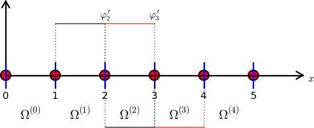
The \( \basphi_i(x) \) function is a hat function with peak at \( x=\xno{i} \) and a linear variation in \( [\xno{i-1},\xno{i}] \) and \( [\xno{i},\xno{i+1}] \). The derivative is \( 1/h \) to the left of \( \xno{i} \) and \( -1/h \) to the right, or more formally, $$ \begin{equation} \basphi_i'(x) = \left\lbrace\begin{array}{ll} 0, & x < \xno{i-1},\\ h^{-1}, & \xno{i-1} \leq x < \xno{i},\\ -h^{-1}, & \xno{i} \leq x < \xno{i+1},\\ 0, & x\geq \xno{i+1} \end{array} \right. \tag{55} \end{equation} $$ Figure 2 shows \( \basphi_2'(x) \) and \( \basphi_3'(x) \).
Figure 2: Illustration of the derivative of piecewise linear basis functions associated with nodes in cell 2.
We realize that \( \basphi_i' \) and \( \basphi_j' \) have no overlap, and hence their product vanishes, unless \( i \) and \( j \) are nodes belonging to the same cell. The only nonzero contributions to the coefficient matrix are therefore $$ \begin{align*} A_{i-1,i-2} &=\int_0^L\basphi_i'(x) \basphi_{i-1}'(x) \dx,\\ A_{i-1,i-1}&=\int_0^L\basphi_{i}'(x)^2 \dx, \\ A_{i-1,i}&=\int_0^L\basphi_{i}'(x)\basphi_{i+1}'(x) \dx, \end{align*} $$ for \( i=1,\ldots,N+1 \), but for \( i=1 \), \( A_{i-1,i-2} \) is not defined, and for \( i=N+1 \), \( A_{i-1,i} \) is not defined.
From Figure 2, we see that \( \basphi_{i-1}'(x) \) and \( \basphi_i'(x) \) have overlap of one cell \( \Omega^{(i-1)}=[\xno{i-1},\xno{i}] \) and that their product then is \( -1/h^{2} \). The integrand is constant and therefore \( A_{i-1,i-2}=-h^{-2}h=-h^{-1} \). A similar reasoning can be applied to \( A_{i-1,i} \), which also becomes \( -h^{-1} \). The integral of \( \basphi_i'(x)^2 \) gets contributions from two cells, \( \Omega^{(i-1)}=[\xno{i-1},\xno{i}] \) and \( \Omega^{(i)}=[\xno{i},\xno{i+1}] \), but \( \basphi_i'(x)^2=h^{-2} \) in both cells, and the length of the integration interval is \( 2h \) so we get \( A_{i-1,i-1}=2h^{-1} \).
The right-hand side involves an integral of \( 2\basphi_i(x) \), \( i=1,\ldots,N_n-2 \), which is just the area under a hat function of height 1 and width \( 2h \), i.e., equal to \( h \). Hence, \( b_{i-1}=2h \).
To summarize the linear system, we switch from \( i \) to \( i+1 \) such that we can write $$ A_{i,i-1}=A_{i,i+1}=-h^{-1},\quad A_{i,i}=2h^{-1},\quad b_i = 2h\tp$$
The equation system to be solved only involves the unknowns \( c_i \) for \( i\in\If \). With our numbering of unknowns and nodes, we have that \( c_i \) equals \( u(\xno{i+1}) \). The complete matrix system then takes the following form: $$ \begin{equation} \frac{1}{h}\left( \begin{array}{ccccccccc} 2 & -1 & 0 &\cdots & \cdots & \cdots & \cdots & \cdots & 0 \\ -1 & 2 & -1 & \ddots & & & & & \vdots \\ 0 & -1 & 2 & -1 & \ddots & & & & \vdots \\ \vdots & \ddots & & \ddots & \ddots & 0 & & & \vdots \\ \vdots & & \ddots & \ddots & \ddots & \ddots & \ddots & & \vdots \\ \vdots & & & 0 & -1 & 2 & -1 & \ddots & \vdots \\ \vdots & & & & \ddots & \ddots & \ddots &\ddots & 0 \\ \vdots & & & & &\ddots & \ddots &\ddots & -1 \\ 0 &\cdots & \cdots &\cdots & \cdots & \cdots & 0 & -1 & 2 \end{array} \right) \left( \begin{array}{c} c_0 \\ \vdots\\ \vdots\\ \vdots \\ \vdots \\ \vdots \\ \vdots \\ \vdots\\ c_{N} \end{array} \right) = \left( \begin{array}{c} 2h \\ \vdots\\ \vdots\\ \vdots \\ \vdots \\ \vdots \\ \vdots \\ \vdots\\ 2h \end{array} \right) \tag{56} \end{equation} $$
A typical row in the matrix system (56) can be written as $$ \begin{equation} -\frac{1}{h}c_{i-1} + \frac{2}{h}c_{i} - \frac{1}{h}c_{i+1} = 2h\tp \tag{57} \end{equation} $$ Let us introduce the notation \( u_j \) for the value of \( u \) at node \( j \): \( u_j=u(\xno{j}) \), since we have the interpretation \( u(\xno{j})=\sum_jc_j\basphi(\xno{j})=\sum_j c_j\delta_{ij}=c_j \). The unknowns \( c_0,\ldots,c_N \) are \( u_1,\ldots,u_{N_n-2} \). Shifting \( i \) with \( i+1 \) in (57) and inserting \( u_i = c_{i-1} \), we get $$ \begin{equation} -\frac{1}{h}u_{i-1} + \frac{2}{h}u_{i} - \frac{1}{h}u_{i+1} = 2h, \tag{58} \end{equation} $$
A finite difference discretization of \( -u''(x)=2 \) by a centered, second-order finite difference approximation \( u''(x_i)\approx [D_x D_x u]_i \) with \( \Delta x = h \) yields $$ \begin{equation} -\frac{u_{i-1} - 2u_{i} + u_{i+1}}{h^2} = 2, \tag{59} \end{equation} $$ which is, in fact, equivalent to (58) if (58) is divided by \( h \). Therefore, the finite difference and the finite element method are equivalent in this simple test problem.
Sometimes a finite element method generates the finite difference equations on a uniform mesh, and sometimes the finite element method generates equations that are different. The differences are modest, but may influence the numerical quality of the solution significantly, especially in time-dependent problems. It depends on the problem at hand whether a finite element discretization is more or less accurate than a corresponding finite difference discretization.
Software for finite element computations normally employs the cell by cell computational procedure where an element matrix and vector are calculated for each cell and assembled in the global linear system. Let us go through the details of this type of algorithm.
All integrals are mapped to the local reference coordinate system \( X\in [-1,1] \). In the present case, the matrix entries contain derivatives with respect to \( x \), $$ \begin{equation*} A_{i-1,j-1}^{(e)}=\int_{\Omega^{(e)}} \basphi_i'(x)\basphi_j'(x) \dx = \int_{-1}^1 \frac{d}{dx}\refphi_r(X)\frac{d}{dx}\refphi_s(X) \frac{h}{2} \dX, \end{equation*} $$ where the global degree of freedom \( i \) is related to the local degree of freedom \( r \) through \( i=q(e,r) \). Similarly, \( j=q(e,s) \). The local degrees of freedom run as \( r,s=0,1 \) for a P1 element.
There are simple formulas for the basis functions \( \refphi_r(X) \) as functions of \( X \). However, we now need to find the derivative of \( \refphi_r(X) \) with respect to \( x \). Given $$ \refphi_0(X)=\half(1-X),\quad\refphi_1(X)=\half(1+X), $$ we can easily compute \( d\refphi_r/ dX \): $$ \frac{d\refphi_0}{dX} = -\half,\quad \frac{d\refphi_1}{dX} = \half\tp $$ From the chain rule, $$ \begin{equation} \frac{d\refphi_r}{dx} = \frac{d\refphi_r}{dX}\frac{dX}{dx} = \frac{2}{h}\frac{d\refphi_r}{dX}\tp \tag{60} \end{equation} $$ The transformed integral is then $$ \begin{equation*} A_{i-1,j-1}^{(e)}=\int_{\Omega^{(e)}} \basphi_i'(x)\basphi_j'(x) \dx = \int_{-1}^1 \frac{2}{h}\frac{d\refphi_r}{dX}\frac{2}{h}\frac{d\refphi_s}{dX} \frac{h}{2} \dX \tp \end{equation*} $$
The right-hand side is transformed according to $$ \begin{equation*} b_{i-1}^{(e)} = \int_{\Omega^{(e)}} 2\basphi_i(x) \dx = \int_{-1}^12\refphi_r(X)\frac{h}{2} \dX,\quad i=q(e,r),\ r=0,1 \tp \end{equation*} $$
Specifically for P1 elements we arrive at the following calculations for the element matrix entries: $$ \begin{align*} \tilde A_{0,0}^{(e)} &= \int_{-1}^1\frac{2}{h}\left(-\half\right) \frac{2}{h}\left(-\half\right)\frac{h}{2} \dX = \frac{1}{h}\\ \tilde A_{0,1}^{(e)} &= \int_{-1}^1\frac{2}{h}\left(-\half\right) \frac{2}{h}\left(\half\right)\frac{h}{2} \dX = -\frac{1}{h}\\ \tilde A_{1,0}^{(e)} &= \int_{-1}^1\frac{2}{h}\left(\half\right) \frac{2}{h}\left(-\half\right)\frac{h}{2} \dX = -\frac{1}{h}\\ \tilde A_{1,1}^{(e)} &= \int_{-1}^1\frac{2}{h}\left(\half\right) \frac{2}{h}\left(\half\right)\frac{h}{2} \dX = \frac{1}{h} \end{align*} $$ The element vector entries become $$ \begin{align*} \tilde b_0^{(e)} &= \int_{-1}^12\half(1-X)\frac{h}{2} \dX = h\\ \tilde b_1^{(e)} &= \int_{-1}^12\half(1+X)\frac{h}{2} \dX = h\tp \end{align*} $$ Expressing these entries in matrix and vector notation, we have $$ \begin{equation} \tilde A^{(e)} =\frac{1}{h}\left(\begin{array}{rr} 1 & -1\\ -1 & 1 \end{array}\right),\quad \tilde b^{(e)} = h\left(\begin{array}{c} 1\\ 1 \end{array}\right)\tp \tag{61} \end{equation} $$
The first and last cell involve only one unknown and one basis function because of the Dirichlet boundary conditions at the first and last node. The element matrix therefore becomes a \( 1\times 1 \) matrix and there is only one entry in the element vector. On cell 0, only \( \baspsi_0=\basphi_1 \) is involved, corresponding to integration with \( \refphi_1 \). On cell \( N_e \), only \( \baspsi_N=\basphi_{N_n-2} \) is involved, corresponding to integration with \( \refphi_0 \). We then get the special end-cell contributions $$ \begin{equation} \tilde A^{(e)} =\frac{1}{h}\left(\begin{array}{r} 1 \end{array}\right),\quad \tilde b^{(e)} = h\left(\begin{array}{c} 1 \end{array}\right), \tag{62} \end{equation} $$ for \( e=0 \) and \( e=N_e \). In these cells, we have only one degree of freedom, not two as in the interior cells.
The next step is to assemble the contributions from the various cells. The assembly of an element matrix and vector into the global matrix and right-hand side can be expressed as $$ A_{q(e,r),q(e,s)} = A_{q(e,r),q(e,s)} + \tilde A^{(e)}_{r,s},\quad b_{q(e,r)} = b_{q(e,r)} + \tilde b^{(e)}_{r},\quad $$ for \( r \) and \( s \) running over all local degrees of freedom in cell \( e \).
To make the assembly algorithm more precise, it is convenient to set up Python data structures and a code snippet for carrying out all details of the algorithm. For a mesh of four equal-sized P1 elements and \( L=2 \) we have
vertices = [0, 0.5, 1, 1.5, 2]
cells = [[0, 1], [1, 2], [2, 3], [3, 4]]
dof_map = [[0], [0, 1], [1, 2], [2]]
The total number of degrees of freedom is 3, being the function
values at the internal 3 nodes where \( u \) is unknown.
In cell 0 we have global degree of freedom 0, the next
cell has \( u \) unknown at its two nodes, which become
global degrees of freedom 0 and 1, and so forth according to
the dof_map list. The mathematical \( q(e,r) \) quantity is nothing
but the dof_map list.
Assume all element matrices are stored in a list Ae such that
Ae[e][i,j] is \( \tilde A_{i,j}^{(e)} \). A corresponding list
for the element vectors is named be, where be[e][r] is
\( \tilde b_r^{(e)} \).
A Python code snippet
illustrates all details of the assembly algorithm:
# A[i,j]: coefficient matrix, b[i]: right-hand side
for e in range(len(Ae)):
    for r in range(Ae[e].shape[0]):
        for s in range(Ae[e].shape[1]):
            A[dof_map[e,r],dof_map[e,s]] += Ae[e][i,j]
        b[dof_map[e,r]] += be[e][i,j]
The general case with N_e P1 elements of length h has
N_n = N_e + 1
vertices = [i*h for i in range(N_n)]
cells = [[e, e+1] for e in range(N_e)]
dof_map = [[0]] + [[e-1, e] for i in range(1, N_e)] + [[N_n-2]]
Carrying out the assembly results in a linear system that is identical to (56), which is not surprising, since the procedures is mathematically equivalent to the calculations in the physical domain.
So far, our technique for computing the matrix system have assumed that \( u(0)=u(L)=0 \). The next section deals with the extension to nonzero Dirichlet conditions.