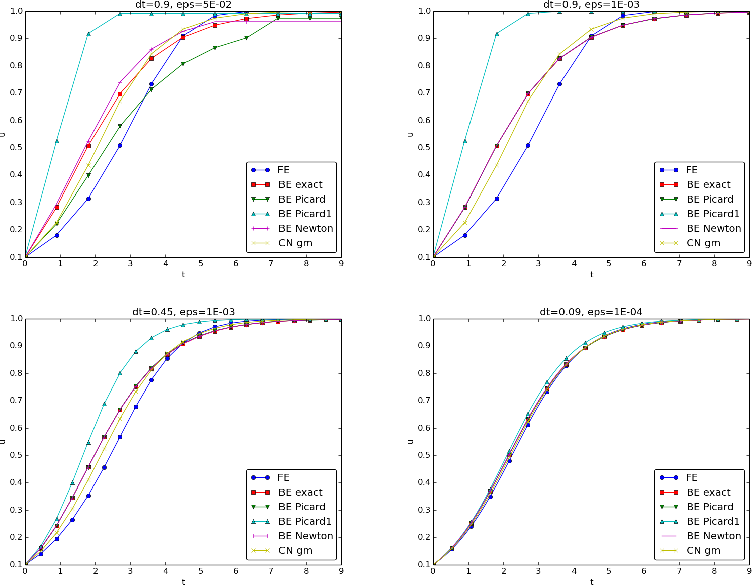
Figure 1: The impact of solution strategies and for four different time step lengths on the solution.
What makes differential equations nonlinear?
Examples on linear and nonlinear differential equations
Introduction of basic concepts
The scaled logistic ODE
Linearization by explicit time discretization
An implicit method: Backward Euler discretization
Detour: new notation
Exact solution of quadratic nonlinear equations
How do we pick the right solution in this case?
Linearization
Picard iteration
The algorithm of Picard iteration
The algorithm of Picard iteration with classical math notation
Stopping criteria
A single Picard iteration
Implicit Crank-Nicolson discretization
Linearization by a geometric mean
Newton's method
Newton's method with an iteration index
Using Newton's method on the logistic ODE
Using Newton's method on the logistic ODE with typical math notation
Relaxation may improve the convergence
Implementation; part 1
Implementation; part 2
Implementation; part 3
Experiments: accuracy of iteration methods
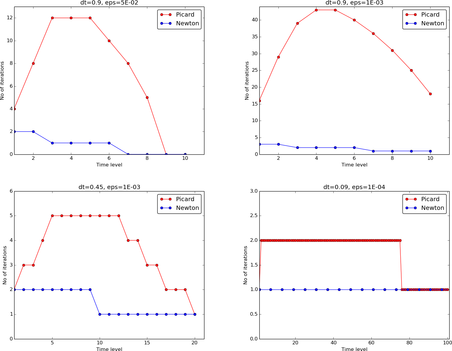
Experiments: number of iterations
The effect of relaxation can potentially be great!
Generalization to a general nonlinear ODE
Explicit time discretization
Backward Euler discretization
Picard iteration for Backward Euler scheme
Manual linearization for a given \( f(u,t) \)
Computational experiments with partially implicit treatment of \( f \)
Newton's method for Backward Euler scheme
Crank-Nicolson discretization
Picard and Newton iteration in the Crank-Nicolson case
Systems of ODEs
A Backward Euler scheme for the vector ODE \( u^{\prime}=f(u,t) \)
Example: Crank-Nicolson scheme for the oscillating pendulum model
The nonlinear \( 2\times 2 \) system
Systems of nonlinear algebraic equations
Notation for general systems of algebraic equations
Picard iteration
Algorithm for relaxed Picard iteration
Newton's method for \( F(u)=0 \)
Algorithm for Newton's method
Newton's method for \( A(u)u=b(u) \)
Comparison of Newton and Picard iteration
Combined Picard-Newton algorithm
Stopping criteria
Combination of absolute and relative stopping criteria
Example: A nonlinear ODE model from epidemiology
Implicit time discretization
A Picard iteration
Newton's method
Actually no need to bother with nonlinear algebraic equations for this particular model...
Linearization at the differential equation level
PDE problem
Explicit time integration
Backward Euler scheme
Picard iteration for Backward Euler scheme
Picard iteration with alternative notation
Backward Euler scheme and Newton's method
Calculation details of Newton's method at the PDE level
Calculation details of Newton's method at the PDE level
Result of Newton's method at the PDE level
Similarity with Picard iteration
Using new notation for implementation
Combined Picard and Newton formulation
Crank-Nicolson discretization
Arithmetic means: which variant is best?
Solution of nonlinear equations in the Crank-Nicolson scheme
Discretization of 1D stationary nonlinear differential equations
Relevance of this stationary 1D problem
Finite difference discretizations
Finite difference scheme
Boundary conditions
The structure of the equation system
The equation for the Neumann boundary condition
The equation for the Dirichlet boundary condition
Nonlinear equations for a mesh with two cells
Picard iteration
The matrix systems to be solved
Newton's method; Jacobian (1)
Newton's method; Jacobian (2)
Newton's method; nonlinear equations at the end points
Galerkin-type discretizations
The nonlinear algebraic equations
Fundamental integration problem: how to deal with \( \int f(\sum_kc_k\baspsi_k)\baspsi_idx \) for unknown \( c_k \)?
We choose \( \baspsi_i \) as finite element basis functions
The group finite element method
What is the point with the group finite element method?
Simplified problem for symbolic calculations
Integrating very simple nonlinear functions results in complicated expressions in the finite element method
Application of the group finite element method
Lumping the mass matrix gives finite difference form
Alternative: evaluation of finite element terms at nodes gives great simplifications
Numerical integration of nonlinear terms
Finite elements for a variable coefficient Laplace term
Numerical integration at the nodes
Summary of finite element vs finite difference nonlinear algebraic equations
Real computations utilize accurate numerical integration
Picard iteration defined from the variational form
The linear system in Picard iteration
The equations in Newton's method
Useful formulas for computing the Jacobian
Computing the Jacobian
Computations in a reference cell \( [-1,1] \)
How to handle Dirichlet conditions in Newton's method
Multi-dimensional PDE problems
Backward Euler and variational form
Nonlinear algebraic equations arising from the variational form
A note on our notation and the different meanings of \( u \) (1)
A note on our notation and the different meanings of \( u \) (2)
Newton's method (1)
Newton's method (2)
Non-homogeneous Neumann conditions
Robin condition
Finite difference discretization in a 2D problem
Picard iteration
Newton's method: the nonlinear algebraic equations
Newton's method: the Jacobian and its sparsity
Newton's method: details of the Jacobian
Good exercise at this point: \( J_{i,j,i,j} \)
Continuation methods
Continuation method: solve difficult problem as a sequence of simpler problems
Example on a continuation method
Linear ODE: $$ u^{\prime} (t) = a(t)u(t) + b(t)$$
Nonlinear ODE: $$ u^{\prime}(t) = u(t)(1 - u(t)) = u(t) - {\color{red}u(t)^2}$$
This (pendulum) ODE is also nonlinear: $$ u^{\prime\prime} + \gamma\sin u = 0$$ because $$ \sin u = u - \frac{1}{6}u^3 + \Oof{u^5},$$ contains products of \( u \)
Forward Euler method: $$ \frac{u^{n+1} - u^n}{\Delta t} = u^n(1 - u^n)$$
gives a linear algebraic equation for the unknown value \( u^{n+1} \)!
Explicit time integration methods will (normally) linearize a nonlinear problem.
Another example: 2nd-order Runge-Kutta method $$ \begin{align*} u^* &= u^n + \Delta t u^n(1 - u^n),\\ u^{n+1} &= u^n + \Delta t \half \left( u^n(1 - u^n) + u^*(1 - u^*)) \right)\tp \end{align*} $$
A backward time difference $$ \frac{u^{n} - u^{n-1}}{\Delta t} = u^n(1 - u^n) $$
gives a nonlinear algebraic equation for the unknown \( u^n \). The equation is of quadratic type (which can easily be solved exactly): $$ \Delta t (u^n)^2 + (1-\Delta t)u^n - u^{n-1} = 0 $$
To make formulas less overloaded and the mathematics as close as possible to computer code, a new notation is introduced:
Solution of \( F(u)=0 \): $$ u = \frac{1}{2\Delta t} \left(-1+\Delta t \pm \sqrt{(1-\Delta t)^2 + 4\Delta t u^{(1)}}\right) $$
Nonlinear algebraic equations may have multiple solutions!
Let's investigate the nature of the two roots:
>>> import sympy as sym
>>> dt, u_1, u = sym.symbols('dt u_1 u')
>>> r1, r2 = sym.solve(dt*u**2 + (1-dt)*u - u_1, u)  # find roots
>>> r1
(dt - sqrt(dt**2 + 4*dt*u_1 - 2*dt + 1) - 1)/(2*dt)
>>> r2
(dt + sqrt(dt**2 + 4*dt*u_1 - 2*dt + 1) - 1)/(2*dt)
>>> print r1.series(dt, 0, 2)
-1/dt + 1 - u_1 + dt*(u_1**2 - u_1) + O(dt**2)
>>> print r2.series(dt, 0, 2)
u_1 + dt*(-u_1**2 + u_1) + O(dt**2)
The r1 root behaves as \( 1/\Delta t\rightarrow\infty \)
as \( \Delta t\rightarrow 0 \)! Therefore, only the r2 root is of
relevance.
Nonliner equation from Backward Euler scheme for logistic ODE: $$ F(u) = au^2 + bu + c = 0$$
Let \( u^{-} \) be an available approximation of the unknown \( u \).
Linearization of \( u^2 \): \( u^{-}u \) $$ F(u)\approx\hat F(u) = au^{-}u + bu + c = 0$$
But
At a time level, set \( u^{-}=u^{(1)} \) (solution at previous time level) and iterate: $$ u = -\frac{c}{au^{-} + b},\quad u^{-}\ \leftarrow\ u$$
This technique is known as
Or with a time level \( n \) too: $$ au^{n,k} u^{n,k+1} + bu^{n,k+1} - u^{n-1} = 0\quad\Rightarrow\quad u^{n,k+1} = \frac{u^{n-1}}{au^{n,k} + b},\quad k=0,1,\ldots$$
Using change in solution: $$ |u - u^{-}| \leq\epsilon_u$$
or change in residual: $$ |F(u)|= |au^2+bu + c| < \epsilon_r$$
Common simple and cheap technique: perform 1 single Picard iteration $$ \frac{u^{n} - u^{n-1}}{\Delta t} = u^n(1 - {\color{red}u^{n-1}}) $$
Inconsistent time discretization (\( u(1-u) \) must be evaluated for \( n \), \( n-1 \), or \( n-\frac{1}{2} \)) - can produce quite inaccurate results, but is very popular.
Crank-Nicolson discretization: $$ [D_t u = u(1-u)]^{n+\half}$$ $$ \frac{u^{n+1}-u^n}{\Delta t} = u^{n+\half} - (u^{n+\half})^2 $$
Approximate \( u^{n+\half} \) as usual by an arithmetic mean, $$ u^{n+\half}\approx \half(u^n + u^{n+1})$$ $$ (u^{n+\half})^2\approx \frac{1}{4}(u^n + u^{n+1})^2\quad\hbox{(nonlinear term)}$$
which is nonlinear in the unknown \( u^{n+1} \).
Using a geometric mean for \( (u^{n+\half})^2 \) linearizes the nonlinear term \( (u^{n+\half})^2 \) (error \( \Oof{\Delta t^2} \) as in the discretization of \( u^{\prime} \)): $$ (u^{n+\half})^2\approx u^nu^{n+1}$$
Arithmetic mean on the linear \( u^{n+\frac{1}{2}} \) term and a geometric mean for \( (u^{n+\half})^2 \) gives a linear equation for \( u^{n+1} \): $$ \frac{{\color{red}u^{n+1}}-u^n}{\Delta t} = \half(u^n + {\color{red}u^{n+1}}) - u^n{\color{red}u^{n+1}}$$
Note: Here we turned a nonlinear algebraic equation into a linear one. No need for iteration! (Consistent \( \Oof{\Delta t^2} \) approx.)
Write the nonlinear algebraic equation as $$ F(u) = 0 $$
Newton's method: linearize \( F(u) \) by two terms from the Taylor series, $$ \begin{align*} F(u) &= F(u^{-}) + F^{\prime}(u^{-})(u - u^{-}) + {\half}F^{\prime\prime}(u^{-})(u-u^{-})^2 +\cdots\\ & \approx F(u^{-}) + F^{\prime}(u^{-})(u - u^{-}) \equiv \hat F(u) \end{align*} $$
The linear equation \( \hat F(u)=0 \) has the solution $$ u = u^{-} - \frac{F(u^{-})}{F^{\prime}(u^{-})}$$
Note that \( \hat F \) in Picard and Newton are different!
Newton's method exhibits quadratic convergence if \( u^k \) is sufficiently close to the solution. Otherwise, the method may diverge.
The iteration method becomes $$ u = u^{-} - \frac{a(u^{-})^2 + bu^{-} + c}{2au^{-} + b},\quad u^{-}\ \leftarrow u $$
Start of iteration: \( u^{-}=u^{(1)} \)
Set iteration start as \( u^{n,0}= u^{n-1} \) and iterate with explicit indices for time (\( n \)) and Newton iteration (\( k \)): $$ u^{n,k+1} = u^{n,k} - \frac{\Delta t (u^{n,k})^2 + (1-\Delta t)u^{n,k} - u^{n-1}} {2\Delta t u^{n,k} + 1 - \Delta t} $$
Compare notation with $$ u = u^{-} - \frac{\Delta t (u^{-})^2 + (1-\Delta t)u^{-} - u^{(1)}} {2\Delta t u^{-} + 1 - \Delta t} $$
Simple formula when used in Newton's method: $$ u = u^{-} - \omega \frac{F(u^{-})}{F^{\prime}(u^{-})} $$
Program logistic.py
def BE_logistic(u0, dt, Nt, choice='Picard',
                eps_r=1E-3, omega=1, max_iter=1000):
    if choice == 'Picard1':
        choice = 'Picard';  max_iter = 1

    u = np.zeros(Nt+1)
    iterations = []
    u[0] = u0
    for n in range(1, Nt+1):
        a = dt
        b = 1 - dt
        c = -u[n-1]

        if choice == 'Picard':

            def F(u):
                return a*u**2 + b*u + c

            u_ = u[n-1]
            k = 0
            while abs(F(u_)) > eps_r and k < max_iter:
                u_ = omega*(-c/(a*u_ + b)) + (1-omega)*u_
                k += 1
            u[n] = u_
            iterations.append(k)
def BE_logistic(u0, dt, Nt, choice='Picard',
                eps_r=1E-3, omega=1, max_iter=1000):
    ...
        elif choice == 'Newton':

            def F(u):
                return a*u**2 + b*u + c

            def dF(u):
                return 2*a*u + b

            u_ = u[n-1]
            k = 0
            while abs(F(u_)) > eps_r and k < max_iter:
                u_ = u_ - omega*F(u_)/dF(u_)
                k += 1
            u[n] = u_
            iterations.append(k)
    return u, iterations
The Crank-Nicolson method with a geometric mean:
def CN_logistic(u0, dt, Nt):
    u = np.zeros(Nt+1)
    u[0] = u0
    for n in range(0, Nt):
        u[n+1] = (1 + 0.5*dt)/(1 + dt*u[n] - 0.5*dt)*u[n]
    return u
Figure 1: The impact of solution strategies and for four different time step lengths on the solution.
Figure 2: Comparison of the number of iterations at various time levels for Picard and Newton iteration.
| \( \Delta t \) | \( \epsilon_r \) | Picard | Newton |
|---|---|---|---|
| \( 0.2 \) | \( 10^{-7} \) | 5 | 2 |
| \( 0.2 \) | \( 10^{-3} \) | 2 | 1 |
| \( 0.4 \) | \( 10^{-7} \) | 12 | 3 |
| \( 0.4 \) | \( 10^{-3} \) | 4 | 2 |
| \( 0.8 \) | \( 10^{-7} \) | 58 | 3 |
| \( 0.8 \) | \( 10^{-3} \) | 4 | 2 |
Note: \( f \) is in general nonlinear in \( u \) so the ODE is nonlinear
Forward Euler and all explicit methods sample \( f \) with known values and all nonlinearities are gone: $$ \frac{{\color{red}u^{n+1}}-u^n}{\Delta t} = f(u^n, t_n) $$
Backward Euler \( [D_t^- u = f]^n \) leads to nonlinear algebraic equations: $$ F(u^n) = u^{n} - \Delta t\, f(u^n, t_n) - u^{n-1}=0$$
Alternative notation: $$ F(u) = u - \Delta t\, f(u, t_n) - u^{(1)} = 0$$
A simple Picard iteration, not knowing anything about the nonlinear structure of \( f \), must approximate \( f(u,t_n) \) by \( f(u^{-},t_n) \): $$ \hat F(u) = u - \Delta t\, f(u^{-},t_n) - u^{(1)}$$
The iteration starts with \( u^{-}=u^{(1)} \) and proceeds with repeating $$ u^* = \Delta t\, f(u^{-},t_n) + u^{(1)},\quad u = \omega u^* + (1-\omega)u^{-}, \quad u^{-}\ \leftarrow\ u$$ until a stopping criterion is fulfilled.
(Idea: \( u\approx u^{-} \))
Newton's method requires the computation of the derivative $$ F^{\prime}(u) = 1 - \Delta t\frac{\partial f}{\partial u}(u,t_n)$$
Start with \( u^{-}=u^{(1)} \), then iterate $$ u = u^{-} - \omega \frac{F(u^{-})}{F^{\prime}(u^{-})} = u^{-} - \omega \frac{u^{-} - \Delta t\, f(u^{-},t_{n}) -u^{(1)}}{1 - \Delta t \frac{\partial}{\partial u}f(u^{-},t_n)} $$
The standard Crank-Nicolson scheme with arithmetic mean approximation of \( f \) reads $$ \frac{u^{n+1} - u^n}{\Delta t} = \half(f(u^{n+1}, t_{n+1}) + f(u^n, t_n))$$
Nonlinear algebraic equation: $$ F(u) = u - u^{(1)} - \Delta t{\half}f(u,t_{n+1}) - \Delta t{\half}f(u^{(1)},t_{n}) = 0 $$
Picard iteration (for a general \( f \)): $$ \hat F(u) = u - u^{(1)} - \Delta t{\half}f(u^{-},t_{n+1}) - \Delta t{\half}f(u^{(1)},t_{n})$$
Newton's method: $$ F(u) = u - u^{(1)} - \Delta t{\half}f(u,t_{n+1}) - \Delta t{\half}f(u^{(1)},t_{n}) $$ $$ F^{\prime}(u)= 1 - \half\Delta t\frac{\partial f}{\partial u}(u,t_{n+1})$$
Introduce vector notation:
Strategy: apply scalar scheme to each component
This can be written more compactly in vector form as $$ \frac{u^n- u^{n-1}}{\Delta t} = f(u^n,t_n)$$
This is a system of nonlinear algebraic equations, $$ u^n - \Delta t\,f(u^n,t_n) - u^{n-1}=0,$$ or written out $$ \begin{align*} u_0^n - \Delta t\, f_0(u^n,t_n) - u_0^{n-1} &= 0,\\ &\vdots\\ u_N^n - \Delta t\, f_N(u^n,t_n) - u_N^{n-1} &= 0\tp \end{align*} $$
The scaled equations for an oscillating pendulum: $$ \begin{align} \dot\omega &= -\sin\theta -\beta \omega |\omega|, \label{_auto1}\\ \dot\theta &= \omega, \label{_auto2} \end{align} $$
Set \( u_0=\omega \), \( u_1=\theta \) $$ \begin{align*} u_0^{\prime} = f_0(u,t) &= -\sin u_1 - \beta u_0|u_0|,\\ u_1^{\prime} = f_1(u,t) &= u_0\tp \end{align*} $$
Crank-Nicolson discretization: $$ \begin{align} \frac{u_0^{n+1}-u_0^{n}}{\Delta t} &= -\sin u_1^{n+\frac{1}{2}} - \beta u_0^{n+\frac{1}{2}}|u_0^{n+\frac{1}{2}}| \approx -\sin\left(\frac{1}{2}(u_1^{n+1} + u_1^n)\right) - \beta\frac{1}{4} (u_0^{n+1} + u_0^n)|u_0^{n+1}+u_0^n|, \label{_auto3}\\ \frac{u_1^{n+1}-u_1^n}{\Delta t} &= u_0^{n+\frac{1}{2}}\approx \frac{1}{2} (u_0^{n+1}+u_0^n)\tp \label{_auto4} \end{align} $$
Introduce \( u_0 \) and \( u_1 \) for \( u_0^{n+1} \) and \( u_1^{n+1} \), write \( u_0^{(1)} \) and \( u_1^{(1)} \) for \( u_0^n \) and \( u_1^n \), and rearrange: $$ \begin{align*} F_0(u_0,u_1) &= {\color{red}u_0} - u_0^{(1)} + \Delta t\,\sin\left(\frac{1}{2}({\color{red}u_1} + u_1^{(1)})\right) + \frac{1}{4}\Delta t\beta ({\color{red}u_0} + u_0^{(1)}) |{\color{red}u_0} + u_0^{(1)}| =0 \\ F_1(u_0,u_1) &= {\color{red}u_1} - u_1^{(1)} -\frac{1}{2}\Delta t({\color{red}u_0} + u_0^{(1)}) =0 \end{align*} $$
Systems of nonlinear algebraic equations arise from solving systems of ODEs or solving PDEs
where $$ u=(u_0,\ldots,u_N),\quad F=(F_0,\ldots,F_N)$$
Special linear system-type structure
(arises frequently in PDE problems):
$$ A(u)u = b(u)$$
Picard iteration for \( F(u)=0 \) is meaningless unless there is some structure that we can linearize. For \( A(u)u=b(u) \) we can linearize $$ A(u^{-})u = b(u^{-})$$
Note: we solve a system of nonlinear algebraic equations as a sequence of linear systems.
Given \( A(u)u=b(u) \) and an initial guess \( u^{-} \), iterate until convergence:
"Until convergence": \( ||u - u^{-}|| \leq \epsilon_u \) or \( ||A(u)u-b|| \leq\epsilon_r \)
Linearization of \( F(u)=0 \) equation via multi-dimensional Taylor series: $$ F(u) = F(u^{-}) + J(u^{-}) \cdot (u - u^{-}) + \mathcal{O}(||u - u^{-}||^2) $$
where \( J \) is the Jacobian of \( F \), sometimes denoted \( \nabla_uF \), defined by $$ J_{i,j} = \frac{\partial F_i}{\partial u_j}$$
Approximate the original nonlinear system \( F(u)=0 \) by $$ \hat F(u) = F(u^{-}) + J(u^{-}) \cdot \delta u =0,\quad \delta u = u - u^{-}$$
which is linear vector equation in \( u \)
Solution by a two-step procedure:
For $$ F_i = \sum_k A_{i,k}(u)u_k - b_i(u)$$
one gets $$ J_{i,j} = \frac{\partial F_i}{\partial u_j} = A_{i,j}+\sum_k \frac{\partial A_{i,k}}{\partial u_j}u_k - \frac{\partial b_i}{\partial u_j} $$
Matrix form: $$ (A + A^{\prime}u - b^{\prime})\delta u = -Au + b$$ $$ (A(u^{-}) + A^{\prime}(u^{-})u^{-} - b^{\prime}(u^{-}))\delta u = -A(u^{-})u^{-} + b(u^{-})$$
Newton: $$ (A(u^{-}) + A^{\prime}(u^{-})u^{-} - b^{\prime}(u^{-}))\delta u = -A(u^{-})u^{-} + b(u^{-})$$
Rewrite: $$ \underbrace{A(u^{-})(u^{-}+\delta u) - b(u^{-})}_{\hbox{Picard system}} +\, \gamma (A^{\prime}(u^{-})u^{-} - b^{\prime}(u^{-}))\delta u = 0$$
All the "Picard terms" are contained in the Newton formulation.
Write a common Picard-Newton algorithm so we can trivially switch between the two methods (e.g., start with Picard, get faster convergence with Newton when \( u \) is closer to the solution)
Given \( A(u) \), \( b(u) \), and an initial guess \( u^{-} \), iterate until convergence:
Let \( ||\cdot|| \) be the standard Eucledian vector norm. Several termination criteria are much in use:
Problem with relative criterion: a small \( ||F(u_0)|| \) (because \( u_0\approx u \), perhaps because of small \( \Delta t \)) must be significantly reduced. Better with absolute criterion.
Spreading of a disease (e.g., a flu) can be modeled by a \( 2\times 2 \) ODE system $$ \begin{align*} S^{\prime} &= -\beta SI\\ I^{\prime} &= \beta SI - \nu I \end{align*} $$
Here:
A Crank-Nicolson scheme: $$ \begin{align*} \frac{S^{n+1}-S^n}{\Delta t} &= -\beta [SI]^{n+\half} \approx -\frac{\beta}{2}(S^nI^n + S^{n+1}I^{n+1})\\ \frac{I^{n+1}-I^n}{\Delta t} &= \beta [SI]^{n+\half} - \nu I^{n+\half} \approx \frac{\beta}{2}(S^nI^n + S^{n+1}I^{n+1}) - \frac{\nu}{2}(I^n + I^{n+1}) \end{align*} $$
New notation: \( S \) for \( S^{n+1} \), \( S^{(1)} \) for \( S^n \), \( I \) for \( I^{n+1} \), \( I^{(1)} \) for \( I^n \) $$ \begin{align*} F_S(S,I) &= S - S^{(1)} + \half\Delta t\beta(S^{(1)}I^{(1)} + SI) = 0\\ F_I(S,I) &= I - I^{(1)} - \half\Delta t\beta(S^{(1)}I^{(1)} + SI) + \half\Delta t\nu(I^{(1)} + I) =0 \end{align*} $$
Jacobian: $$ J = \left(\begin{array}{cc} \frac{\partial}{\partial S} F_S & \frac{\partial}{\partial I}F_S\\ \frac{\partial}{\partial S} F_I & \frac{\partial}{\partial I}F_I \end{array}\right) = \left(\begin{array}{cc} 1 + \half\Delta t\beta I & \half\Delta t\beta S\\ - \half\Delta t\beta I & 1 - \half\Delta t\beta S + \half\Delta t\nu \end{array}\right) $$
Newton system: \( J(u^{-})\delta u = -F(u^{-}) \) $$ \begin{align*} & \left(\begin{array}{cc} 1 + \half\Delta t\beta I^{-} & \half\Delta t\beta S^{-}\\ - \half\Delta t\beta I^{-} & 1 - \half\Delta t\beta S^{-} + \half\Delta t\nu \end{array}\right) \left(\begin{array}{c} \delta S\\ \delta I \end{array}\right) =\\ & \qquad\qquad \left(\begin{array}{c} S^{-} - S^{(1)} + \half\Delta t\beta(S^{(1)}I^{(1)} + S^{-}I^{-})\\ I^{-} - I^{(1)} - \half\Delta t\beta(S^{(1)}I^{(1)} + S^{-}I^{-}) - \half\Delta t\nu(I^{(1)} + I^{-}) \end{array}\right) \end{align*} $$
For this particular system of ODEs, explicit time integration methods work very well. Even a Forward Euler scheme is fine, but the 4-th order Runge-Kutta method is an excellent balance between high accuracy, high efficiency, and simplicity.
Goal: linearize a PDE like $$ \frac{\partial u}{\partial t} = \nabla\cdot ({\color{red}\dfc(u)\nabla u}) + {\color{red}f(u)} $$
Forward Euler method: $$ [D_t^+ u = \nabla\cdot (\dfc(u)\nabla u) + f(u)]^n$$ $$ \frac{u^{n+1} - u^n}{\Delta t} = \nabla\cdot (\dfc(u^n)\nabla u^n) + f(u^n)$$
This is a linear equation in the unknown \( u^{n+1}(\x) \), with solution $$ u^{n+1} = u^n + \Delta t\nabla\cdot (\dfc(u^n)\nabla u^n) + \Delta t f(u^n) $$
Disadvantage: \( \Delta t \leq (\max\alpha)^{-1}(\Delta x^2 + \Delta y^2 + \Delta z^2) \)
Backward Euler scheme: $$ [D_t^- u = \nabla\cdot (\dfc(u)\nabla u) + f(u)]^n$$
Written out: $$ \frac{u^{n} - u^{n-1}}{\Delta t} = \nabla\cdot (\dfc(u^n)\nabla u^n) + f(u^n) $$
This is a nonlinear, stationary PDE for the unknown function \( u^n(\x) \)
We have $$ \frac{u^{n} - u^{n-1}}{\Delta t} = \nabla\cdot (\dfc(u^n)\nabla u^n) + f(u^n) $$
Picard iteration: $$ \frac{u^{n,k+1} - u^{n-1}}{\Delta t} = \nabla\cdot (\dfc(u^{n,k}) \nabla u^{n,k+1}) + f(u^{n,k}) $$
Start iteration with \( u^{n,0}=u^{n-1} \)
Rewrite with a simplified, implementation-friendly notation:
Start iteration with \( u^{-}=u^{(1)} \); update with \( u^{-} \) to \( u \).
Let \( u^{n,k} \) be the most recently computed approximation to the unknown \( u^n \). We seek a better approximation $$ u^{n} = u^{n,k} + \delta u $$
Insert \( u^{n,k} +\delta u \) for \( u^n \) in PDE: $$ \frac{u^{n,k} +\delta u - u^{n-1}}{\Delta t} = \nabla\cdot (\dfc(u^{n,k} + \delta u)\nabla (u^{n,k}+\delta u)) + f(u^{n,k}+\delta u) $$
Taylor expand \( \dfc(u^{n,k} + \delta u) \) and \( f(u^{n,k}+\delta u) \): $$ \begin{align*} \dfc(u^{n,k} + \delta u) & = \dfc(u^{n,k}) + \frac{d\dfc}{du}(u^{n,k}) \delta u + \Oof{\delta u^2}\approx \dfc(u^{n,k}) + \dfc^{\prime}(u^{n,k})\delta u\\ f(u^{n,k}+\delta u) &= f(u^{n,k}) + \frac{df}{du}(u^{n,k})\delta u + \Oof{\delta u^2}\approx f(u^{n,k}) + f^{\prime}(u^{n,k})\delta u \end{align*} $$
Inserting linear approximations of \( \dfc \) and \( f \): $$ \begin{align*} \frac{u^{n,k} +\delta u - u^{n-1}}{\Delta t} &= \nabla\cdot (\dfc(u^{n,k})\nabla u^{n,k}) + f(u^{n,k}) + \\ &\quad \nabla\cdot (\dfc(u^{n,k})\nabla \delta u) + \nabla\cdot (\dfc^{\prime}(u^{n,k})\delta u\nabla u^{n,k}) + \\ &\quad \nabla\cdot (\dfc^{\prime}(u^{n,k})\underbrace{\delta u\nabla \delta u}_{\mbox{dropped}}) + f^{\prime}(u^{n,k})\delta u \end{align*} $$
Note: \( \dfc^{\prime}(u^{n,k})\delta u\nabla \delta u \) is \( \Oof{\delta u^2} \) and therefore omitted.
with $$ \begin{align*} F(u^{n,k}) &= \frac{u^{n,k} - u^{n-1}}{\Delta t} - \nabla\cdot (\dfc(u^{n,k})\nabla u^{n,k}) - f(u^{n,k}) \\ \delta F(\delta u; u^{n,k}) &= \frac{1}{\Delta t}\delta u - \nabla\cdot (\dfc(u^{n,k})\nabla \delta u) - \\ &\qquad \nabla\cdot (\dfc^{\prime}(u^{n,k})\delta u\nabla u^{n,k}) - f^{\prime}(u^{n,k})\delta u \end{align*} $$
Note:
Rewrite the PDE for \( \delta u \) using \( u^{n,k} + \delta u =u^{n,k+1} \): $$ \begin{align*} & \frac{u^{n,k+1} - u^{n-1}}{\Delta t} = \nabla\cdot (\dfc(u^{n,k})\nabla u^{n,k+1}) + f(u^{n,k})\\ &\qquad + \nabla\cdot (\dfc^{\prime}(u^{n,k})\delta u\nabla u^{n,k}) + f^{\prime}(u^{n,k})\delta u \end{align*} $$
Note:
Observe:
Crank-Nicolson discretization applies a centered difference at \( t_{n+\frac{1}{2}} \): $$ [D_t u = \nabla\cdot (\dfc(u)\nabla u) + f(u)]^{n+\frac{1}{2}}\tp$$
Many choices of formulating an arithmetic mean: $$ \begin{align*} [f(u)]^{n+\frac{1}{2}} &\approx f(\frac{1}{2}(u^n + u^{n+1})) = [f(\overline{u}^t)]^{n+\frac{1}{2}}\\ [f(u)]^{n+\frac{1}{2}} &\approx \frac{1}{2}(f(u^n) + f(u^{n+1})) =[\overline{f(u)}^t]^{n+\frac{1}{2}}\\ [\dfc(u)\nabla u]^{n+\frac{1}{2}} &\approx \dfc(\frac{1}{2}(u^n + u^{n+1}))\nabla (\frac{1}{2}(u^n + u^{n+1})) = \dfc(\overline{u}^t)\nabla \overline{u}^t]^{n+\frac{1}{2}}\\ [\dfc(u)\nabla u]^{n+\frac{1}{2}} &\approx \frac{1}{2}(\dfc(u^n) + \dfc(u^{n+1}))\nabla (\frac{1}{2}(u^n + u^{n+1})) = [\overline{\dfc(u)}^t\nabla\overline{u}^t]^{n+\frac{1}{2}}\\ [\dfc(u)\nabla u]^{n+\frac{1}{2}} &\approx \frac{1}{2}(\dfc(u^n)\nabla u^n + \dfc(u^{n+1})\nabla u^{n+1}) = [\overline{\dfc(u)\nabla u}^t]^{n+\frac{1}{2}} \end{align*} $$
Is there any differences in accuracy between
It can be shown (by Taylor series around \( t_{n+\frac{1}{2}} \)) that both approximations are \( \Oof{\Delta t^2} \)
No big difference from the Backward Euler case, just more terms:
Differential equation: $$ -(\dfc(u)u^{\prime})^{\prime} + au = f(u),\quad x\in (0,L) $$
Boundary conditions: $$ \dfc(u(0))u^{\prime}(0) = C,\quad u(L)=D $$
1. As stationary limit of a diffusion PDE $$ u_t = (\alpha(u)u_x)_x + au + f(u) $$
(\( u_t\rightarrow 0 \))
2. The time-discrete problem at each time level arising from a Backward Euler scheme for a diffusion PDE $$ u_t = (\alpha(u)u_x)_x + f(u) $$
(\( au \) comes from \( u_t \), \( a\sim 1/\Delta t \), \( f(u) + u^{n-1}/\Delta t \) becomes \( f(u) \) in the model problem)
The nonlinear term \( (\dfc(u)u^{\prime})^{\prime} \) behaves just as a variable coefficient term \( (\dfc(x)u^{\prime})^{\prime} \) wrt discretization: $$ [-D_x\dfc D_x u +au = f]_i$$
Written out at internal points: $$ \begin{align*} -\frac{1}{\Delta x^2} \left(\dfc_{i+\half}(u_{i+1}-u_i) - \dfc_{i-\half}(u_{i}-u_{i-1})\right) + au_i &= f(u_i) \end{align*} $$
\( \dfc_{i+\half} \): two choices $$ \begin{align*} \dfc_{i+\half} &\approx \dfc(\half(u_i + u_{i+1})) = [\dfc(\overline{u}^x)]^{i+\half} \\ \dfc_{i+\half} &\approx \half(\dfc(u_i) + \dfc(u_{i+1})) = [\overline{\dfc(u)}^x]^{i+\half} \end{align*} $$
results in $$ [-D_x\overline{\dfc}^x D_x u +au = f]_i\tp$$ $$ \begin{align*} &-\frac{1}{2\Delta x^2} \left((\dfc(u_i)+\dfc(u_{i+1}))(u_{i+1}-u_i) - (\dfc(u_{i-1})+\dfc(u_{i}))(u_{i}-u_{i-1})\right)\\ &\qquad\qquad + au_i = f(u_i) \end{align*} $$
The fictitious value \( u_{-1} \) can, as usual, be eliminated with the aid of the scheme at \( i=0 \)
Structure of nonlinear algebraic equations: $$ A(u)u = b(u)$$ $$ \begin{align*} A_{i,i} &= \frac{1}{2\Delta x^2}(\dfc(u_{i-1}) + 2\dfc(u_{i}) +\dfc(u_{i+1})) + a\\ A_{i,i-1} &= -\frac{1}{2\Delta x^2}(\dfc(u_{i-1}) + \dfc(u_{i}))\\ A_{i,i+1} &= -\frac{1}{2\Delta x^2}(\dfc(u_{i}) + \dfc(u_{i+1}))\\ b_i &= f(u_i) \end{align*} $$
Note:
For \( i=0 \): insert $$ u_{-1} = u_1 -\frac{2\Delta x}{\dfc(u_0)} $$ into the numerical scheme, leading to a modified expression for \( A_{0,0} \). The expression for \( A_{i,i+1} \) remains the same for \( i=0 \), and \( A_{i,i-1} \) for \( i=0 \) does not enter the system.
1. For \( i=N_x \) we can use the Dirichlet condition as a separate equation $$ u_i = D,\quad i=N_x$$
2. Alternative: we can substitute \( u_{N_x} \) by \( D \) in the numerical scheme for \( i=N_x-1 \) and do not use a seperate equation for \( u_{N_x} \).
Let's do all the details! We omit a separate equation for the \( u=D \) condition at \( i=N_x \). Starting point is then $$ \begin{align*} A_{0,-1}u_{-1} + A_{0,0}u_0 + A_{0,1}u_1 &= b_0\\ A_{1,0}u_{0} + A_{1,1}u_1 + A_{1,2}u_2 &= b_1 \end{align*} $$
Must
Use the most recently computed vaue \( u^{-} \) of \( u \) in \( A(u) \) and \( b(u) \): $$ A(u^{-})u = b(u^{-})$$ $$ \begin{align*} \frac{1}{2\Delta x^2}(& -(\dfc(u^-_{-1}) + 2\dfc(u^-_{0}) + \dfc(u^-_{1}))u_1\, +\\ &(\dfc(u^-_{-1}) + 2\dfc(u^-_{0}) + \dfc(u^-_{1}))u_0 + au_0\\ &=f(u^-_0) - \frac{1}{\dfc(u^-_0)\Delta x}(\dfc(u^-_{-1}) + \dfc(u^-_{0}))C, \end{align*} $$ $$ \begin{align*} \frac{1}{2\Delta x^2}(&-(\dfc(u^-_{0}) + \dfc(u^-_{1}))u_{0}\, +\\ & (\dfc(u^-_{0}) + 2\dfc(u^-_{1}) + \dfc(D))u_1 + au_1\\ &=f(u^-_1) + \frac{1}{2\Delta x^2}(\dfc(u^-_{1}) + \dfc(D))D\tp \end{align*} $$
Eliminating the Dirichlet condition at \( i=N_x \): $$ \left(\begin{array}{cc} B_{0,0}& B_{0,1}\\ B_{1,0} & B_{1,1} \end{array}\right) \left(\begin{array}{c} u_0\\ u_1 \end{array}\right) = \left(\begin{array}{c} d_0\\ d_1 \end{array}\right) $$
Including the equation for \( i=N_x \): $$ \left(\begin{array}{ccc} B_{0,0}& B_{0,1} & 0\\ B_{1,0} & B_{1,1} & B_{1,2}\\ 0 & 0 & 1 \end{array}\right) \left(\begin{array}{c} u_0\\ u_1\\ u_2 \end{array}\right) = \left(\begin{array}{c} d_0\\ d_1^{*}\\ D \end{array}\right) $$
Nonlinear eq.no \( i \) has the structure $$ \begin{align*} F_i &= A_{i,i-1}(u_{i-1},u_i)u_{i-1} + A_{i,i}(u_{i-1},u_i,u_{i+1})u_i +\\ &\qquad A_{i,i+1}(u_i, u_{i+1})u_{i+1} - b_i(u_i) \end{align*} $$
Need Jacobian, i.e., need to differentiate \( F(u)=A(u)u - b(u) \) wrt \( u \). Example: $$ \begin{align*} &\frac{\partial}{\partial u_i}(A_{i,i}(u_{i-1},u_i,u_{i+1})u_i) = \frac{\partial A_{i,i}}{\partial u_i}u_i + A_{i,i} \frac{\partial u_i}{\partial u_i}\\ &\quad = \frac{\partial}{\partial u_i}( \frac{1}{2\Delta x^2}(\dfc(u_{i-1}) + 2\dfc(u_{i}) +\dfc(u_{i+1})) + a)u_i +\\ &\qquad\frac{1}{2\Delta x^2}(\dfc(u_{i-1}) + 2\dfc(u_{i}) +\dfc(u_{i+1})) + a\\ &\quad =\frac{1}{2\Delta x^2}(2\dfc^\prime (u_i)u_i +\dfc(u_{i-1}) + 2\dfc(u_{i}) +\dfc(u_{i+1})) + a \end{align*} $$
The complete Jacobian becomes (make sure you get this!) $$ \begin{align*} J_{i,i} &= \frac{\partial F_i}{\partial u_i} = \frac{\partial A_{i,i-1}}{\partial u_i}u_{i-1} + \frac{\partial A_{i,i}}{\partial u_i}u_i + A_{i,i} + \frac{\partial A_{i,i+1}}{\partial u_i}u_{i+1} - \frac{\partial b_i}{\partial u_{i}}\\ &= \frac{1}{2\Delta x^2}( -\dfc^{\prime}(u_i)u_{i-1} +2\dfc^{\prime}(u_i)u_{i} +\dfc(u_{i-1}) + 2\dfc(u_i) + \dfc(u_{i+1})) +\\ &\quad a -\frac{1}{2\Delta x^2}\dfc^{\prime}(u_{i})u_{i+1} - b^{\prime}(u_i)\\ J_{i,i-1} &= \frac{\partial F_i}{\partial u_{i-1}} = \frac{\partial A_{i,i-1}}{\partial u_{i-1}}u_{i-1} + A_{i-1,i} + \frac{\partial A_{i,i}}{\partial u_{i-1}}u_i - \frac{\partial b_i}{\partial u_{i-1}}\\ &= \frac{1}{2\Delta x^2}( -\dfc^{\prime}(u_{i-1})u_{i-1} - (\dfc(u_{i-1}) + \dfc(u_i)) + \dfc^{\prime}(u_{i-1})u_i)\\ J_{i,i+1} &= \frac{\partial A_{i,i+1}}{\partial u_{i-1}}u_{i+1} + A_{i+1,i} + \frac{\partial A_{i,i}}{\partial u_{i+1}}u_i - \frac{\partial b_i}{\partial u_{i+1}}\\ &=\frac{1}{2\Delta x^2}( -\dfc^{\prime}(u_{i+1})u_{i+1} - (\dfc(u_{i}) + \dfc(u_{i+1})) + \dfc^{\prime}(u_{i+1})u_i) \end{align*} $$
At \( i=0 \), replace \( u_{-1} \) by formula from Neumann condition.
Note: The size of the Jacobian depends on 1 or 2.
Insert Neumann condition: $$ [\dfc(u)u^{\prime}v]_0^L = \dfc(u(L))u^{\prime}(L)v(L) - \dfc(u(0))u^{\prime}(0)v(0) = -Cv(0) $$
Find \( u\in V \) such that $$ \int_0^L \dfc(u)u^{\prime}v^{\prime}\dx + \int_0^L auv\dx = \int_0^L f(u)v\dx - Cv(0),\quad \forall v\in V $$
\( \forall v\in V\ \Rightarrow\ \forall i\in\If \), \( v=\baspsi_i \). Inserting \( u=D+\sum_jc_j\baspsi_j \) and sorting terms: $$ \sum_{j}\left( \int\limits_0^L \left(\dfc(D+\sum_{k}c_k\baspsi_k) \baspsi_j^{\prime}\baspsi_i^{\prime} + a \baspsi_j\baspsi_i\right)\dx\right)c_j = \int\limits_0^L f(D+\sum_{k}c_k\baspsi_k)\baspsi_i\dx - C\baspsi_i(0) $$
This is a nonlinear algebraic system
Degree of freedom number \( \nu(i) \) in the mesh corresponds to unknown number \( i \) (\( c_i \)).
Model problem: \( \nu(i)=i \), \( \If=\{0,\ldots,N_n-2\} \) (last node excluded) $$ u = D + \sum_{j\in\If} c_j\basphi_{\nu(j)}$$
or with \( \basphi_i \) in the boundary function: $$ u = D\basphi_{N_n-1} + \sum_{j\in\If} c_j\basphi_{j}$$
Since \( u \) is represented by \( \sum_j\basphi_j u(\xno{j}) \), we may use the same approximation for \( f(u) \): $$ f(u)\approx \sum_{j} f(\xno{j})\basphi_j $$
\( f(\xno{j}) \): value of \( f \) at node \( j \). With \( u_j \) as \( u(\xno{j}) \), we can write $$ f(u)\approx \sum_{j} f(u_{j})\basphi_j $$
This approximation is known as the group finite element method or the product approximation technique. The index \( j \) runs over all node numbers in the mesh.
Simple nonlinear problem: \( -u^{\prime\prime}=u^2 \), \( u'(0)=1 \), \( u'(L)=0 \). $$ \int_0^L u^{\prime}v^{\prime}\dx = \int_0^L u^2v\dx - v(0),\quad\forall v\in V$$
Now,
Consider \( \int u^2v\dx \) with \( u = \sum_ku_k\basphi_k \) and \( v=\basphi_i \): $$ \int_0^L (\sum_ku_k\basphi_k)^2\basphi_i\dx$$
Tedious exact evaluation on uniform P1 elements: $$ \frac{h}{12}(u_{i-1}^2 + 2u_i(u_{i-1} + u_{i+1}) + 6u_i^2 + u_{i+1}^2)$$
Finite difference counterpart: \( u_i^2 \) (!)
Corresponding part of difference equation for P1 elements: $$ \frac{h}{6}(f(u_{i-1}) + 4f(u_i) + f(u_{i+1}))$$
Rewrite as "finite difference form plus something": $$ \frac{h}{6}(f(u_{i-1}) + 4f(u_i) + f(u_{i+1})) = h[{\color{red}f(u)} - \frac{h^2}{6}D_xD_x f(u)]_i$$
This is like the finite difference discretization of \( -u'' = f(u) - \frac{h^2}{6}f''(u) \)
Idea: integrate \( \int f(u)v\dx \) numerically with a rule that samples \( f(u)v \) at the nodes only. This involves great simplifications, since $$ \sum_k u_k\basphi_k(\xno{\ell}) = u_\ell$$
and $$ f\basphi_i(\xno{\ell}) = f(\sum_k u_k\underbrace{\basphi_k(\xno{\ell})}_{\delta_{k\ell}}) \underbrace{\basphi_i(\xno{\ell})}_{\delta_{i\ell}} = f(u_\ell)\delta_{i\ell}\quad \neq 0\mbox{ only for } f(u_i)$$
(\( \delta_{ij}=0 \) if \( i\neq j \) and \( \delta_{ij}=1 \) if \( i=j \))
Trapezoidal rule with the nodes only gives the finite difference form of \( [f(u)]_i \): $$ \int_0^L f(\sum_k u_k\basphi_k)(x)\basphi_i(x)\dx \approx h\sum_{\ell=0}^{N_n-1} f(u_\ell)\delta_{i\ell} - \mathcal{C} = h{\color{red}f(u_i)} $$
(\( \mathcal{C} \): boundary adjustment of rule, \( i=0,N_n-1 \))
Consider the term \( (\dfc u^{\prime})^{\prime} \), with the group finite element method: \( \dfc(u)\approx \sum_k\alpha(u_k)\basphi_k \), and the variational counterpart $$ \int_0^L \dfc(\sum_k c_k\basphi_k)\basphi_i^{\prime}\basphi_j^{\prime}\dx \approx \sum_k (\int_0^L \basphi_k\basphi_i^{\prime}\basphi_j^{\prime}\dx) \dfc(u_k) = \ldots $$
Further calculations (see text) lead to $$ -\frac{1}{h}(\half(\dfc(u_i) + \dfc(u_{i+1}))(u_{i+1}-u_i) - \half(\dfc(u_{i-1}) + \dfc(u_{i}))(u_{i}-u_{i-1})) $$
= standard finite difference discretization of \( -(\dfc(u)u^{\prime})^{\prime} \) with an arithmetic mean of \( \dfc(u) \)
Instead of the group finite element method and exact integration, use Trapezoidal rule in the nodes for \( \int_0^L \dfc(\sum_k u_k\basphi_k)\basphi_i^{\prime}\basphi_j^{\prime}\dx \).
Work at the cell level (most convenient with discontinuous \( \basphi_i' \)): $$ \begin{align*} & \int_{-1}^1 \alpha(\sum_t\tilde u_t\refphi_t)\refphi_r'\refphi_s'\frac{h}{2}dX = \int_{-1}^1 \dfc(\sum_{t=0}^1 \tilde u_t\refphi_t)\frac{2}{h}\frac{d\refphi_r}{dX} \frac{2}{h}\frac{d\refphi_s}{dX}\frac{h}{2}dX\\ &\quad = \frac{1}{2h}(-1)^r(-1)^s \int_{-1}^1 \dfc(\sum_{t=0}^1 u_t\refphi_t(X))dX \\ & \qquad \approx \frac{1}{2h}(-1)^r(-1)^s\dfc ( \sum_{t=0}^1\refphi_t(-1)\tilde u_t) + \dfc(\sum_{t=0}^1\refphi_t(1)\tilde u_t)\\ &\quad = \frac{1}{2h}(-1)^r(-1)^s(\dfc(\tilde u_0) + \dfc(\tilde u^{(1)})) \end{align*} $$
Uniform P1 finite elements:
Variational form (\( v=\baspsi_i \)): $$ F_i = \int_0^L \dfc(u)u^{\prime}\baspsi_i^{\prime}\dx + \int_0^L au\baspsi_i\dx - \int_0^L f(u)\baspsi_i\dx + C\baspsi_i(0) = 0 $$
Picard iteration: use "old value" \( u^{-} \) in \( \dfc(u) \) and \( f(u) \) and integrate numerically: $$ F_i = \int_0^L (\dfc(u^{-})u^{\prime}\baspsi_i^{\prime} + au\baspsi_i)\dx - \int_0^L f(u^{-})\baspsi_i\dx + C\baspsi_i(0) $$
This is a linear problem \( a(u,v)=L(v) \) with bilinear and linear forms $$ a(u,v) = \int_0^L (\dfc(u^{-})u^{\prime}v^{\prime} + auv)\dx,\quad L(v) = \int_0^L f(u^{-})v\dx - Cv(0)$$
The linear system now is computed the standard way.
Easy to evaluate right-hand side \( -F_i(u^{-}) \) by numerical integration: $$ F_i = \int_0^L (\dfc(u^{-})u^{\prime}\baspsi_i^{\prime} + au\baspsi_i - f(u^{-})\baspsi_i)\dx + C\baspsi_i(0)=0 $$
(just known functions)
Use \( \dfc^{\prime}(u^{-}) \), \( \dfc(u^{-}) \), \( f^\prime (u^{-}) \), \( f(u^{-}) \) and integrate expressions numerically (only known functions)
\( r,s\in\Ifd \) (local degrees of freedom)
Backward Euler time discretization: $$ u^n - \Delta t\nabla\cdot(\dfc(u^n)\nabla u^n) - \Delta t f(u^n) = u^{n-1}$$
Alternative notation (\( u \) for \( u^n \), \( u^{(1)} \) for \( u^{n-1} \)): $$ u - \Delta t\nabla\cdot(\dfc(u)\nabla u) - \Delta t f(u) = u^{(1)}$$
Boundary conditions: \( \partial u/\partial n=0 \) for simplicity. Variational form: $$ \int_\Omega (uv + \Delta t\,\dfc(u)\nabla u\cdot\nabla v - \Delta t f(u)v - u^{(1)} v)\dx = 0 $$
Picard iteration: $$ F_i \approx \hat F_i = \int_\Omega (u\baspsi_i + \Delta t\,\dfc(u^{-})\nabla u\cdot\nabla \baspsi_i - \Delta t f(u^{-})\baspsi_i - u^{(1)}\baspsi_i)\dx = 0 $$
This is a variable coefficient problem like \( au - \nabla\cdot\dfc(\x)\nabla u = f(\x,t) \) and results in a linear system
PDE problem: \( u(\x,t) \) is the exact solution of $$ u_t = \nabla\cdot(\dfc(u)\nabla u) + f(u) $$
Time discretization: \( u(\x) \) is the exact solution of the time-discrete spatial equation $$ u - \Delta t\nabla\cdot(\dfc(u^n)\nabla u) - \Delta t f(u) = u^{(1)}$$
The same \( u(\x) \) is the exact solution of the (continuous) variational form: $$ \int_\Omega (uv + \Delta t\,\dfc(u)\nabla u\cdot\nabla v - \Delta t f(u)v - u^{(1)} v)\dx,\quad\forall v\in V $$
Or we may approximate \( u \): \( u(\x) = \sum_jc_j\baspsi_j(\x) \) and let this spatially discrete \( u \) enter the variational form, $$ \int_\Omega (uv + \Delta t\,\dfc(u)\nabla u\cdot\nabla v - \Delta t f(u)v - u^{(1)} v)\dx,\quad\forall v\in V $$
Picard iteration: \( u(\x) \) solves the approximate variational form $$ \int_\Omega (uv + \Delta t\,\dfc(u^{-})\nabla u\cdot\nabla v - \Delta t f(u^{-})v - u^{(1)} v)\dx $$
Could introduce
Need to evaluate \( F_i(u^{-}) \): $$ F_i \approx \hat F_i = \int_\Omega (u^{-}\baspsi_i + \Delta t\,\dfc(u^{-}) \nabla u^{-}\cdot\nabla \baspsi_i - \Delta t f(u^{-})\baspsi_i - u^{(1)}\baspsi_i)\dx $$
To compute the Jacobian we need $$ \begin{align*} \frac{\partial u}{\partial c_j} &= \sum_k\frac{\partial}{\partial c_j} c_k\baspsi_k = \baspsi_j\\ \frac{\partial \nabla u}{\partial c_j} &= \sum_k\frac{\partial}{\partial c_j} c_k\nabla \baspsi_k = \nabla \baspsi_j \end{align*} $$
The Jacobian becomes $$ \begin{align*} J_{i,j} = \frac{\partial F_i}{\partial c_j} = \int_\Omega & (\baspsi_j\baspsi_i + \Delta t\,\dfc^{\prime}(u)\baspsi_j \nabla u\cdot\nabla \baspsi_i + \Delta t\,\dfc(u)\nabla\baspsi_j\cdot\nabla\baspsi_i - \\ &\ \Delta t f^{\prime}(u)\baspsi_j\baspsi_i)\dx \end{align*} $$
Evaluation of \( J_{i,j} \) as the coefficient matrix in the Newton system \( J\delta u = -F \) means \( J(u^{-}) \): $$ \begin{align*} J_{i,j} = \int_\Omega & (\baspsi_j\baspsi_i + \Delta t\,\dfc^{\prime}(u^{-})\baspsi_j \nabla u^{-}\cdot\nabla \baspsi_i + \Delta t\,\dfc(u^{-})\nabla\baspsi_j\cdot\nabla\baspsi_i - \\ &\ \Delta t f^{\prime}(u^{-})\baspsi_j\baspsi_i)\dx \end{align*} $$
A natural physical flux condition: $$ -\dfc(u)\frac{\partial u}{\partial n} = g,\quad\x\in\partial\Omega_N $$
Integration by parts gives the boundary term $$ \int_{\partial\Omega_N}\dfc(u)\frac{\partial u}{\partial u}v\ds $$
Inserting the nonlinear Neumann condition: $$ -\int_{\partial\Omega_N}gv\ds$$
(no nonlinearity)
Heat conduction problems often apply a kind of Newton's cooling law, also known as a Robin condition, at the boundary: $$ -\dfc(u)\frac{\partial u}{\partial u} = h(u)(u-T_s(t)),\quad\x\in\partial\Omega_R $$
Here:
Use \( h(u^{-})(u-T_s) \) for Picard, differentiate for Newton
Backward Euler in time, centered differences in space: $$ [D_t^- u = D_x\overline{\dfc(u)}^xD_x u + D_y\overline{\dfc(u)}^yD_y u + f(u)]_{i,j}^n $$ $$ \begin{align*} u^n_{i,j} &- \frac{\Delta t}{h^2}( \half(\dfc(u_{i,j}^n) + \dfc(u_{i+1,j}^n))(u_{i+1,j}^n-u_{i,j}^n)\\ &\quad - \half(\dfc(u_{i-1,j}^n) + \dfc(u_{i,j}^n))(u_{i,j}^n-u_{i-1,j}^n) \\ &\quad + \half(\dfc(u_{i,j}^n) + \dfc(u_{i,j+1}^n))(u_{i,j+1}^n-u_{i,j}^n)\\ &\quad - \half(\dfc(u_{i,j-1}^n) + \dfc(u_{i,j}^n))(u_{i,j}^n-u_{i-1,j-1}^n)) - \Delta tf(u_{i,j}^n) = u^{n-1}_{i,j} \end{align*} $$
Nonlinear algebraic system on the form \( A(u)u=b(u) \)
Define the nonlinear equations (use \( u \) for \( u^n \), \( u^{(1)} \) for \( u^{n-1} \)): $$ \begin{align*} F_{i,j} &= u_{i,j} - \frac{\Delta t}{h^2}(\\ &\qquad \half(\dfc(u_{i,j}) + \dfc(u_{i+1,j}))(u_{i+1,j}-u_{i,j}) -\\ &\qquad \half(\dfc(u_{i-1,j}) + \dfc(u_{i,j}))(u_{i,j}-u_{i-1,j}) + \\ &\qquad \half(\dfc(u_{i,j}) + \dfc(u_{i,j+1}))(u_{i,j+1}-u_{i,j}) -\\ &\qquad \half(\dfc(u_{i,j-1}) + \dfc(u_{i,j}))(u_{i,j}-u_{i-1,j-1})) - \Delta t\, f(u_{i,j}) - u^{(1)}_{i,j} = 0 \end{align*} $$
Newton system: $$ \sum_{r\in\Ix}\sum_{s\in\Iy}J_{i,j,r,s}\delta u_{r,s} = -F_{i,j}, \quad i\in\Ix,\ j\in\Iy\tp$$
But \( F_{i,j} \) contains only \( u_{i\pm 1,j} \), \( u_{i,j\pm 1} \), and \( u_{i,j} \). We get nonzero contributions only for \( J_{i,j,i-1,j} \), \( J_{i,j,i+1,j} \), \( J_{i,j,i,j-1} \), \( J_{i,j,i,j+1} \), and \( J_{i,j,i,j} \). The Newton system collapses to $$ \begin{align*} J_{i,j,r,s}\delta u_{r,s} = J_{i,j,i,j}\delta u_{i,j} & + J_{i,j,i-1,j}\delta u_{i-1,j} +\\ & J_{i,j,i+1,j}\delta u_{i+1,j} + J_{i,j,i,j-1}\delta u_{i,j-1} + J_{i,j,i,j+1}\delta u_{i,j+1} \end{align*} $$
Compute \( J_{i,j,i,j} \): $$ \begin{align*} F_{i,j} &= u_{i,j} - \frac{\Delta t}{h^2}(\\ &\qquad \half(\dfc(u_{i,j}) + \dfc(u_{i+1,j}))(u_{i+1,j}-u_{i,j}) -\\ &\qquad \half(\dfc(u_{i-1,j}) + \dfc(u_{i,j}))(u_{i,j}-u_{i-1,j}) + \\ &\qquad \half(\dfc(u_{i,j}) + \dfc(u_{i,j+1}))(u_{i,j+1}-u_{i,j}) -\\ &\qquad \half(\dfc(u_{i,j-1}) + \dfc(u_{i,j}))(u_{i,j}-u_{i-1,j-1})) - \Delta t\, f(u_{i,j}) - u^{(1)}_{i,j} = 0\\ J_{i,j,i,j} &= \frac{\partial F_{i,j}}{\partial u_{i,j}} \end{align*} $$
Pseudo-plastic fluids may be \( q=-0.8 \), which is a difficult problem for Picard/Newton iteration. $$ \Lambda\in [0,1]:\quad q=-\Lambda 0.8 $$ $$ -\nabla\cdot\left( ||\nabla u||^{-\Lambda 0.8}\nabla u\right) = f$$
Start with \( \Lambda = 0 \), increase in steps to \( \Lambda =1 \), use previous solution as initial guess for Newton or Picard