The finite element method is normally used for discretization in space. There are two alternative strategies for performing a discretization in time:

• use finite differences for time derivatives to arrive at a recursive set of spatial problems that can be discretized by the finite element method, or
• discretize in space by finite elements first, and then solve the resulting system of ordinary differential equations (ODEs) by some standard method for ODEs.

We shall exemplify these strategies using a simple diffusion problem

\[\tag{1} \frac{\partial u}{\partial t} = {\alpha}\nabla^2 u + f(\boldsymbol{x}, t),\quad \boldsymbol{x}\in\Omega,\ t\in (0,T],\]

\[\tag{2} u(\boldsymbol{x}, 0) = I(\boldsymbol{x}),\quad \boldsymbol{x}\in\Omega,\]

\[\tag{3} \frac{\partial u}{\partial n} = 0,\quad \boldsymbol{x}\in\partial\Omega,\ t\in (0,T]\]\[ {\thinspace .}\]

Here, \(u(\boldsymbol{x},t)\) is the unknown function, \({\alpha}\) is a constant, and \(f(\boldsymbol{x},t)\) and \(I(x)\) are given functions. We have assigned the particular boundary condition (3) to minimize the details on handling boundary conditions in the finite element method.

Discretization in time by a Forward Euler scheme

Time discretization

We can apply a finite difference method in time to (1). First we need a mesh in time, here taken as uniform with mesh points \(t_n = n\Delta t\), \(n=0,1,\ldots,N_t\). A Forward Euler scheme consists of sampling (1) at \(t_n\) and approximating the time derivative by a forward difference \([D_t^+ u]^n\approx (u^{n+1}-u^n)/\Delta t\). This approximation turns (1) into a differential equation that is discrete in time, but still continuous in space. With a finite difference operator notation we can write the time-discrete problem as

\[\tag{4} [D_t^+ u = {\alpha}\nabla^2 u + f]^n,\]

for \(n=1,2,\ldots,N_t-1\). Writing this equation out in detail and isolating the unknown \(u^{n+1}\) on the left-hand side, demonstrates that the time-discrete problem is a recursive set of problems that are continuous in space:

\[\tag{5} u^{n+1} = u^n + \Delta t \left( {\alpha}\nabla^2 u^n + f(\boldsymbol{x}, t_n)\right)\]\[ {\thinspace .}\]

Given \(u^0=I\), we can use (5) to compute \(u^1,u^2,\dots,u^{N_t}\).

Space discretization

We now introduce a finite element approximation to \({u_{\small\mbox{e}}}^n\) and \({u_{\small\mbox{e}}}^{n+1}\) in (9), where the coefficients depend on the time level:

\[\tag{6} {u_{\small\mbox{e}}}^n \approx u^n = \sum_{j=0}^{N} c_j^{n}{\psi}_j(\boldsymbol{x}),\]

\[\tag{7} {u_{\small\mbox{e}}}^{n+1} \approx u^{n+1} = \sum_{j=0}^{N} c_j^{n+1}{\psi}_j(\boldsymbol{x})\]\[ {\thinspace .}\]

Note that, as before, \(N\) denotes the number of degrees of freedom in the spatial domain. The number of time points is denoted by \(N_t\). We define a space \(V\) spanned by the basis functions \(\left\{ {{\psi}}_i \right\}_{i\in{\mathcal{I}_s}}\).

More precise notation

For absolute clarity in the various stages of the discretizations, we introduce \({u_{\small\mbox{e}}}(\boldsymbol{x},t)\) as the exact solution of the space-and time-continuous partial differential equation (1) and \({u_{\small\mbox{e}}}^n(\boldsymbol{x})\) as the time-discrete approximation, arising from the finite difference method in time (4). More precisely, \({u_{\small\mbox{e}}}\) fulfills

\[ \tag{8} \frac{\partial {u_{\small\mbox{e}}}}{\partial t} = {\alpha}\nabla^2 {u_{\small\mbox{e}}} + f(\boldsymbol{x}, t) ,\]\[ while \( {u_{\small\mbox{e}}}^{n+1} \) , with a superscript, is the solution of the time-discrete equations\]\[.. _Eq:fem:deq:diffu:FE:eq:uex:n:\]

\[ \tag{9} {u_{\small\mbox{e}}}^{n+1} = {u_{\small\mbox{e}}}^n + \Delta t \left( {\alpha}\nabla^2 {u_{\small\mbox{e}}}^n + f(\boldsymbol{x}, t_n)\right)\]\[ {\thinspace .}\]\[ The \( {u_{\small\mbox{e}}}^{n+1} \) quantity is then discretized in space and approximated by \( u^{n+1} \) .\]

Variational forms

A Galerkin method or a weighted residual method with weighting functions \(w_i\) can now be formulated. We insert (6) and (7) in (9) to obtain the residual

\[R = u^{n+1} - u^n - \Delta t \left( {\alpha}\nabla^2 u^n + f(\boldsymbol{x}, t_n)\right) {\thinspace .}\]

The weighted residual principle,

\[\int_\Omega Rw{\, \mathrm{d}x} = 0,\quad \forall w\in W,\]

results in

\[\int_\Omega \left\lbrack u^{n+1} - u^n - \Delta t \left( {\alpha}\nabla^2 u^n + f(\boldsymbol{x}, t_n)\right) \right\rbrack w {\, \mathrm{d}x} =0, \quad\forall w \in W{\thinspace .}\]

From now on we use the Galerkin method so \(W=V\). Isolating the unknown \(u^{n+1}\) on the left-hand side gives

\[\int_{\Omega} u^{n+1}v{\, \mathrm{d}x} = \int_{\Omega} \left\lbrack u^n + \Delta t \left( {\alpha}\nabla^2 u^n + f(\boldsymbol{x}, t_n)\right) \right\rbrack v{\, \mathrm{d}x},\quad \forall v\in V {\thinspace .}\]

As usual in spatial finite element problems involving second-order derivatives, we apply integration by parts on the term \(\int (\nabla^2 u^n)v{\, \mathrm{d}x}\):

\[\int_{\Omega}{\alpha}(\nabla^2 u^n)v {\, \mathrm{d}x} = -\int_{\Omega}{\alpha}\nabla u^n\cdot\nabla v{\, \mathrm{d}x} + \int_{\partial\Omega}{\alpha}\frac{\partial u^n}{\partial n}v {\, \mathrm{d}x} {\thinspace .}\]

The last term vanishes because we have the Neumann condition \(\partial u^n/\partial n=0\) for all \(n\). Our discrete problem in space and time then reads

\[\tag{10} \int_{\Omega} u^{n+1}v{\, \mathrm{d}x} = \int_{\Omega} u^n vdx - \Delta t \int_{\Omega}{\alpha}\nabla u^n\cdot\nabla v{\, \mathrm{d}x} + \Delta t\int_{\Omega}f^n v{\, \mathrm{d}x},\quad \forall \boldsymbol{v}\in V{\thinspace .}\]

This is the variational formulation of our recursive set of spatial problems.

Nonzero Dirichlet boundary conditions

As in stationary problems, we can introduce a boundary function \(B(\boldsymbol{x},t)\) to take care of nonzero Dirichlet conditions:

\[ \tag{11} {u_{\small\mbox{e}}}^n \approx u^n = B(\boldsymbol{x},t_n) + \sum_{j=0}^{N} c_j^{n}{\psi}_j(\boldsymbol{x}),\]\[.. _Eq:fem:deq:diffu:femapprox:np1:B:\]

\[\tag{12} {u_{\small\mbox{e}}}^{n+1} \approx u^{n+1} = B(\boldsymbol{x},t_{n+1}) + \sum_{j=0}^{N} c_j^{n+1}{\psi}_j(\boldsymbol{x})\]\[ {\thinspace .}\]

Simplified notation for the solution at recent time levels

In a program it is only necessary to store \(u^{n+1}\) and \(u^n\) at the same time. It is therefore unnatural to use the index \(n\) in computer code. Instead a natural variable naming is u for \(u^{n+1}\), the new unknown, and u_1 for \(u^n\), the solution at the previous time level. When we have several preceding (already computed) time levels, it is natural to number them like u_1, u_2, u_3, etc., backwards in time. From this notation in software, we introduce a similar mathematical notation to help make the mapping from mathematical formulas to implementation as direct as possible. This principle implies that we let \(u_1\) be the discrete unknown at the previous time level (\(u^{n}\)) and \(u\) represents the discrete unknown at the new time level (\(u^{n+1}\)). Equation (10) with this new naming convention is consequently expressed as

\[\tag{13} \int_{\Omega} u vdx = \int_{\Omega} u_1 vdx - \Delta t \int_{\Omega}{\alpha}\nabla u_1\cdot\nabla v{\, \mathrm{d}x} + \Delta t\int_{\Omega}f^n v{\, \mathrm{d}x} {\thinspace .}\]

This variational form can alternatively be expressed by the inner product notation:

\[\tag{14} (u,v) = (u_1,v) - \Delta t ({\alpha}\nabla u_1,\nabla v) + \Delta t (f^n, v) {\thinspace .}\]

Deriving the linear systems

In the following, we adopt the convention that the unknowns \(c_j^{n+1}\) are written as \(c_j\), while the known \(c_j^n\) from the previous time level are denoted by \(c_{1,j}\). To derive the equations for the new unknown coefficients \(c_j\), we insert

\[u = \sum_{j=0}^{N}c_j{\psi}_j(\boldsymbol{x}),\quad u_1 = \sum_{j=0}^{N} c_{1,j}{\psi}_j(\boldsymbol{x})\]

in (13) or (14), let the equation hold for all \(v={\psi}_i\), \(i=0,\ldots,N\), and order the terms as matrix-vector products:

\[\tag{15} \sum_{j=0}^{N} ({\psi}_i,{\psi}_j) c_j = \sum_{j=0}^{N} ({\psi}_i,{\psi}_j) c_{1,j} -\Delta t \sum_{j=0}^{N} (\nabla{\psi}_i,{\alpha}\nabla{\psi}_j) c_{1,j} + \Delta t (f^n,{\psi}_i),\quad i=0,\ldots,N {\thinspace .}\]

This is a linear system \(\sum_j A_{i,j}c_j = b_i\) with

\[A_{i,j} = ({\psi}_i,{\psi}_j)\]

and

\[b_i = \sum_{j=0}^{N} ({\psi}_i,{\psi}_j) c_{1,j} -\Delta t \sum_{j=0}^{N} (\nabla{\psi}_i,{\alpha}\nabla{\psi}_j) c_{1,j} + \Delta t (f^n,{\psi}_i){\thinspace .}\]

It is instructive and convenient for implementations to write the linear system on the form

\[\tag{16} Mc = Mc_1 - \Delta t Kc_1 + \Delta t f,\]

where

\[\begin{split}M &= \{M_{i,j}\},\quad M_{i,j}=({\psi}_i,{\psi}_j),\quad i,j\in{\mathcal{I}_s},\\ K &= \{K_{i,j}\},\quad K_{i,j}=(\nabla{\psi}_i,{\alpha}\nabla{\psi}_j), \quad i,j\in{\mathcal{I}_s},\\ f &= \{f_i\},\quad f_i=(f(\boldsymbol{x},t_n),{\psi}_i),\quad i\in{\mathcal{I}_s},\\ c &= \{c_i\},\quad i\in{\mathcal{I}_s},\\ c_1 &= \{c_{1,i}\},\quad i\in{\mathcal{I}_s} {\thinspace .}\end{split}\]

We realize that \(M\) is the matrix arising from a term with the zero-th derivative of \(u\), and called the mass matrix, while \(K\) is the matrix arising from a Laplace term \(\nabla^2 u\). The \(K\) matrix is often known as the stiffness matrix. (The terms mass and stiffness stem from the early days of finite elements when applications to vibrating structures dominated. The mass matrix arises from the mass times acceleration term in Newton’s second law, while the stiffness matrix arises from the elastic forces (the “stiffness”) in that law. The mass and stiffness matrix appearing in a diffusion have slightly different mathematical formulas compared to the classic structure problem.)

Remark. The mathematical symbol \(f\) has two meanings, either the function \(f(\boldsymbol{x},t)\) in the PDE or the \(f\) vector in the linear system to be solved at each time level.

Computational algorithm

We observe that \(M\) and \(K\) can be precomputed so that we can avoid computing the matrix entries at every time level. Instead, some matrix-vector multiplications will produce the linear system to be solved. The computational algorithm has the following steps:

1. Compute \(M\) and \(K\).
2. Initialize \(u^0\) by interpolation or projection
3. For \(n=1,2,\ldots,N_t\):

1. compute \(b = Mc_1 - \Delta t Kc_1 + \Delta t f\)
2. solve \(Mc = b\)
3. set \(c_1 = c\)

In case of finite element basis functions, interpolation of the initial condition at the nodes means \(c_{1,j} = I(\boldsymbol{x}_j)\). Otherwise one has to solve the linear system

\[\sum_j{\psi}_j(x_{i})c_{1,j} = I(x_{i}),\]

where \(\boldsymbol{x}_j\) denotes an interpolation point. Projection (or Galerkin’s method) implies solving a linear system with \(M\) as coefficient matrix:

\[\sum_j M_{i,j}c_{1,j} = (I,{\psi}_i),\quad i\in{\mathcal{I}_s}{\thinspace .}\]

Example using sinusoidal basis functions

Let us go through a computational example and demonstrate the algorithm from the previous section. We consider a 1D problem

\[\tag{17} \frac{\partial u}{\partial t} = {\alpha}\frac{\partial^2 u}{\partial x^2},\quad x\in (0,L),\ t\in (0,T],\]

\[\tag{18} u(x, 0) = A\cos(\pi\boldsymbol{x}/L) + B\cos(10\pi x/L),\quad x\in[0,L],\]

\[\tag{19} \frac{\partial u}{\partial x} = 0,\quad x=0,L,\ t\in (0,T]\]\[ {\thinspace .}\]

We use a Galerkin method with basis functions

\[{\psi}_i = \cos(i\pi x/L){\thinspace .}\]

These basis functions fulfill (19), which is not a requirement (there are no Dirichlet conditions in this problem), but helps to make the approximation good.

Since the initial condition (18) lies in the space \(V\) where we seek the approximation, we know that a Galerkin or least squares approximation of the initial condition becomes exact. Therefore,

\[c_{1,1}=A,\quad c_{1,10}=B,\]

while \(c_{1,i}=0\) for \(i\neq 1,10\).

The \(M\) and \(K\) matrices are easy to compute since the basis functions are orthogonal on \([0,L]\). We get

>>> import sympy as sym
>>> x, L = sym.symbols('x L')
>>> i = sym.symbols('i', integer=True)
>>> sym.integrate(sym.cos(i*x*sym.pi/L)**2, (x,0,L))
Piecewise((L, Eq(pi*i/L, 0)), (L/2, True))

which means \(L\) if \(i=0\) and \(L/2\) otherwise. Similarly,

>>> sym.integrate(sym.diff(cos(i*x*sym.pi/L),x)**2, (x,0,L))
pi**2*i**2*Piecewise((0, Eq(pi*i/L, 0)), (L/2, True))/L**2

so

\[\begin{split}M_{0,0}=L,\quad M_{i,i}=L/2,\ i>0,\quad K_{0,0}=0,\quad K_{i,i}=\frac{\pi^2 i^2}{2L},\ i>0{\thinspace .}\end{split}\]

The equation system becomes

\[\begin{split}Lc_0 &= Lc_{1,0} - \Delta t \cdot 0\cdot c_{1,0},\\ \frac{L}{2}c_i &= \frac{L}{2}c_{1,i} - \Delta t \frac{\pi^2 i^2}{2L} c_{1,i},\quad i>0{\thinspace .}\end{split}\]

The first equation always leads to \(c_0=0\) since we start with \(c_{1,0}=0\). The others imply

\[c_i = (1-\Delta t (\frac{\pi i}{L})^2) c_{1,i}{\thinspace .}\]

With the notation \(c^n_i\) for \(c_i\) at the \(n\)-th time level, we can apply the relation above recursively and get

\[c^n_i = (1-\Delta t (\frac{\pi i}{L})^2)^n c^0_i{\thinspace .}\]

Since only two of the coefficients are nonzero at time \(t=0\), we have the closed-form discrete solution

\[u^n_i = A(1-\Delta t (\frac{\pi}{L})^2)^n \cos(\pi x/L) + B(1-\Delta t (\frac{10\pi }{L})^2)^n \cos(10\pi x/L){\thinspace .}\]

Comparing P1 elements with the finite difference method

We can compute the \(M\) and \(K\) matrices using P1 elements in 1D. A uniform mesh on \([0,L]\) is introduced for this purpose. Since the boundary conditions are solely of Neumann type in this sample problem, we have no restrictions on the basis functions \({\psi}_i\) and can simply choose \({\psi}_i = {\varphi}_i\), \(i=0,\ldots,N=N_n-1\).

From the document Stationary variational forms [Ref1] we have that the \(K\) matrix is the same as we get from the finite difference method: \(h[D_xD_x u]^n_i\), while from the section Finite difference interpretation of a finite element approximation in the document Approximation of functions [Ref2] we know that \(M\) can be interpreted as the finite difference approximation \(h[u + \frac{1}{6}h^2D_xD_x u]^n_i\). The equation system \(Mc=b\) in the algorithm is therefore equivalent to the finite difference scheme

\[\tag{20} [D_t^+(u + \frac{1}{6}h^2D_xD_x u) = {\alpha} D_xD_x u + f]^n_i\]\[ {\thinspace .}\]

(More precisely, \(Mc=b\) divided by \(h\) gives the equation above.)

Lumping the mass matrix

As explained in the section Making finite elements behave as finite differences in the document Approximation of functions [Ref2], one can turn the \(M\) matrix into a diagonal matrix \(\hbox{diag}(h/2,h,\ldots,h,h/2)\) by applying the Trapezoidal rule for integration. Then there is no need to solve a linear system at each time level, and the finite element scheme becomes identical to a standard finite difference method

\[\tag{21} [D_t^+ u = {\alpha} D_xD_x u + f]^n_i\]\[ {\thinspace .}\]

The Trapezoidal integration is not as accurate as exact integration and introduces therefore an error. Normally, one thinks of any error as an overall decrease of the accuracy. Nevertheless, errors may cancel each other, and the error introduced by numerical integration may in certain problems lead to improved overall accuracy in the finite element method. The interplay of the errors in the current problem is analyzed in detail in the section Analysis of the discrete equations. The effect of the error is at least not more severe than what is produced by the finite difference method since both are \(\mathcal{O}(h^2)\).

Making \(M\) diagonal is usually referred to as lumping the mass matrix. There is an alternative method to using an integration rule based on the node points: one can sum the entries in each row, place the sum on the diagonal, and set all other entries in the row equal to zero. For P1 elements the methods of lumping the mass matrix give the same result.

Discretization in time by a Backward Euler scheme

Time discretization

The Backward Euler scheme in time applied to our diffusion problem can be expressed as follows using the finite difference operator notation:

\[[D_t^- u = {\alpha}\nabla^2 u + f(\boldsymbol{x}, t)]^n {\thinspace .}\]

Written out, and collecting the unknown \(u^n\) on the left-hand side and all the known terms on the right-hand side, the time-discrete differential equation becomes

\[\tag{22} \boldsymbol{u}^{n} - \Delta t \left( {\alpha}\nabla^2 \boldsymbol{u}^n + f(\boldsymbol{x}, t_{n})\right) = \boldsymbol{u}^{n-1}\]\[ {\thinspace .}\]

Equation (22) can compute \(\boldsymbol{u}^1,\boldsymbol{u}^2,\dots,\boldsymbol{u}^{N_t}\), if we have a start \(\boldsymbol{u}^0=I\) from the initial condition. However, (22) is a partial differential equation in space and needs a solution method based on discretization in space. For this purpose we use an expansion as in (6)-(7).

Variational forms

Inserting (6)-(7) in (22), multiplying by any \(v\in V\) (or \({\psi}_i\in V\)), and integrating by parts, as we did in the Forward Euler case, results in the variational form

\[\tag{23} \int_{\Omega} \left( u^{n}v + \Delta t {\alpha}\nabla u^n\cdot\nabla v\right){\, \mathrm{d}x} = \int_{\Omega} u^{n-1} v{\, \mathrm{d}x} + \Delta t\int_{\Omega}f^n v{\, \mathrm{d}x},\quad\forall v\in V\]\[ {\thinspace .}\]

Expressed with \(u\) as \(u^n\) and \(u_1\) as \(u^{n-1}\), the variational form becomes

\[\tag{24} \int_{\Omega} \left( uv + \Delta t {\alpha}\nabla u\cdot\nabla v\right){\, \mathrm{d}x} = \int_{\Omega} u_1 v{\, \mathrm{d}x} + \Delta t\int_{\Omega}f^n v{\, \mathrm{d}x},\]

or with the more compact inner product notation,

\[\tag{25} (u,v) + \Delta t ({\alpha}\nabla u,\nabla v) = (u_1,v) + \Delta t (f^n,v)\]\[ {\thinspace .}\]

Linear systems

Inserting \(u=\sum_j c_j{\psi}_i\) and \(u_1=\sum_j c_{1,j}{\psi}_i\), and choosing \(v\) to be the basis functions \({\psi}_i\in V\), \(i=0,\ldots,N\), together with doing some algebra, lead to the following linear system to be solved at each time level:

\[\tag{26} (M + \Delta t K)c = Mc_1 + \Delta t f,\]

where \(M\), \(K\), and \(f\) are as in the Forward Euler case. This time we really have to solve a linear system at each time level. The computational algorithm goes as follows.

1. Compute \(M\), \(K\), and \(A=M + \Delta t K\)
2. Initialize \(u^0\) by interpolation or projection
3. For \(n=1,2,\ldots,N_t\):

1. compute \(b = Mc_1 + \Delta t f\)
2. solve \(Ac = b\)
3. set \(c_1 = c\)

In case of finite element basis functions, interpolation of the initial condition at the nodes means \(c_{1,j} = I(\boldsymbol{x}_j)\). Otherwise one has to solve the linear system \(\sum_j{\psi}_j(x_{i})c_j = I(x_{i})\), where \(\boldsymbol{x}_j\) denotes an interpolation point. Projection (or Galerkin’s method) implies solving a linear system with \(M\) as coefficient matrix: \(\sum_j M_{i,j}c_{1,j} = (I,{\psi}_i)\), \(i\in{\mathcal{I}_s}\).

Finite difference operators corresponding to P1 elements

We know what kind of finite difference operators the \(M\) and \(K\) matrices correspond to (after dividing by \(h\)), so (26) can be interpreted as the following finite difference method:

\[\tag{27} [D_t^-(u + \frac{1}{6}h^2D_xD_x u) = {\alpha} D_xD_x u + f]^n_i\]\[ {\thinspace .}\]

The mass matrix \(M\) can be lumped, as explained in the section Comparing P1 elements with the finite difference method, and then the linear system arising from the finite element method with P1 elements corresponds to a plain Backward Euler finite difference method for the diffusion equation:

\[\tag{28} [D_t^- u = {\alpha} D_xD_x u + f]^n_i\]\[ {\thinspace .}\]

Dirichlet boundary conditions

Suppose now that the boundary condition (3) is replaced by a mixed Neumann and Dirichlet condition,

\[\tag{29} u(\boldsymbol{x},t) = u_0(\boldsymbol{x},t),\quad \boldsymbol{x}\in\partial\Omega_D,\]

\[\tag{30} -{\alpha}\frac{\partial}{\partial n} u(\boldsymbol{x},t) = g(\boldsymbol{x},t),\quad \boldsymbol{x}\in\partial{\Omega}_N{\thinspace .}\]

Using a Forward Euler discretization in time, the variational form at a time level becomes

\[\tag{31} \int\limits_\Omega u^{n+1}v{\, \mathrm{d}x} = \int\limits_\Omega (u^n - \Delta t{\alpha}\nabla u^n\cdot\nabla v){\, \mathrm{d}x} + \Delta t\int\limits_\Omega fv {\, \mathrm{d}x} - \Delta t\int\limits_{\partial\Omega_N} gv{\, \mathrm{d}s},\quad \forall v\in V{\thinspace .}\]

Boundary function

The Dirichlet condition \(u=u_0\) at \(\partial\Omega_D\) can be incorporated through a boundary function \(B(\boldsymbol{x})=u_0(\boldsymbol{x})\) and demanding that \(v=0\) at \(\partial\Omega_D\). The expansion for \(u^n\) is written as

\[u^n(\boldsymbol{x}) = u_0(\boldsymbol{x},t_n) + \sum_{j\in{\mathcal{I}_s}}c_j^n{\psi}_j(\boldsymbol{x}){\thinspace .}\]

Inserting this expansion in the variational formulation and letting it hold for all basis functions \({\psi}_i\) leads to the linear system

\[\begin{split}\sum_{j\in{\mathcal{I}_s}} \left(\int\limits_\Omega {\psi}_i{\psi}_j{\, \mathrm{d}x}\right) c^{n+1}_j &= \sum_{j\in{\mathcal{I}_s}} \left(\int\limits_\Omega\left( {\psi}_i{\psi}_j - \Delta t{\alpha}\nabla {\psi}_i\cdot\nabla{\psi}_j\right){\, \mathrm{d}x}\right) c_j^n - \\ &\quad \int\limits_\Omega\left( \left(u_0(\boldsymbol{x},t_{n+1}) - u_0(\boldsymbol{x},t_n)\right) {\psi}_i + \Delta t{\alpha}\nabla u_0(\boldsymbol{x},t_n)\cdot\nabla {\psi}_i\right){\, \mathrm{d}x} \\ & \quad + \Delta t\int\limits_\Omega f{\psi}_i{\, \mathrm{d}x} - \Delta t\int\limits_{\partial\Omega_N} g{\psi}_i{\, \mathrm{d}s}, \quad i\in{\mathcal{I}_s}{\thinspace .}\end{split}\]

Finite element basis functions

When using finite elements, each basis function \({\varphi}_i\) is associated with a node \(x_{i}\). We have a collection of nodes \(\{x_{i}\}_{i\in{I_b}}\) on the boundary \(\partial\Omega_D\). Suppose \(U_k^n\) is the known Dirichlet value at \(x_{k}\) at time \(t_n\) (\(U_k^n=u_0(x_{k},t_n)\)). The appropriate boundary function is then

\[B(\boldsymbol{x},t_n)=\sum_{j\in{I_b}} U_j^n{\varphi}_j{\thinspace .}\]

The unknown coefficients \(c_j\) are associated with the rest of the nodes, which have numbers \(\nu(i)\), \(i\in{\mathcal{I}_s} = \{0,\ldots,N\}\). The basis functions for \(V\) are chosen as \({\psi}_i = {\varphi}_{\nu(i)}\), \(i\in{\mathcal{I}_s}\), and all of these vanish at the boundary nodes as they should. The expansion for \(u^{n+1}\) and \(u^n\) become

\[\begin{split}u^n &= \sum_{j\in{I_b}} U_j^n{\varphi}_j + \sum_{j\in{\mathcal{I}_s}}c_{1,j}{\varphi}_{\nu(j)},\\ u^{n+1} &= \sum_{j\in{I_b}} U_j^{n+1}{\varphi}_j + \sum_{j\in{\mathcal{I}_s}}c_{j}{\varphi}_{\nu(j)}{\thinspace .}\end{split}\]

The equations for the unknown coefficients \(\left\{ {c}_j \right\}_{j\in{\mathcal{I}_s}}\) become

\[\begin{split}\sum_{j\in{\mathcal{I}_s}} \left(\int\limits_\Omega {\varphi}_i{\varphi}_j{\, \mathrm{d}x}\right) c_j &= \sum_{j\in{\mathcal{I}_s}} \left(\int\limits_\Omega\left( {\varphi}_i{\varphi}_j - \Delta t{\alpha}\nabla {\varphi}_i\cdot\nabla{\varphi}_j\right){\, \mathrm{d}x}\right) c_{1,j} - \\ &\quad \sum_{j\in{I_b}}\int\limits_\Omega\left( {\varphi}_i{\varphi}_j(U_j^{n+1} - U_j^n) + \Delta t{\alpha}\nabla {\varphi}_i\cdot\nabla {\varphi}_jU_j^n\right){\, \mathrm{d}x} \\ &\quad + \Delta t\int\limits_\Omega f{\varphi}_i{\, \mathrm{d}x} - \Delta t\int\limits_{\partial\Omega_N} g{\varphi}_i{\, \mathrm{d}s}, \quad i\in{\mathcal{I}_s}{\thinspace .}\end{split}\]

Modification of the linear system

Instead of introducing a boundary function \(B\) we can work with basis functions associated with all the nodes and incorporate the Dirichlet conditions by modifying the linear system. Let \({\mathcal{I}_s}\) be the index set that counts all the nodes: \(\{0,1,\ldots,N=N_n-1\}\). The expansion for \(u^n\) is then \(\sum_{j\in{\mathcal{I}_s}}c^n_j{\varphi}_j\) and the variational form becomes

\[\begin{split}\sum_{j\in{\mathcal{I}_s}} \left(\int\limits_\Omega {\varphi}_i{\varphi}_j{\, \mathrm{d}x}\right) c_j &= \sum_{j\in{\mathcal{I}_s}} \left(\int\limits_\Omega\left( {\varphi}_i{\varphi}_j - \Delta t{\alpha}\nabla {\varphi}_i\cdot\nabla{\varphi}_j\right){\, \mathrm{d}x}\right) c_{1,j} \\ &\quad + \Delta t\int\limits_\Omega f{\varphi}_i{\, \mathrm{d}x} - \Delta t\int\limits_{\partial\Omega_N} g{\varphi}_i{\, \mathrm{d}s}{\thinspace .}\end{split}\]

We introduce the matrices \(M\) and \(K\) with entries \(M_{i,j}=\int\limits_\Omega{\varphi}_i{\varphi}_j{\, \mathrm{d}x}\) and \(K_{i,j}=\int\limits_\Omega{\alpha}\nabla{\varphi}_i\cdot\nabla{\varphi}_j{\, \mathrm{d}x}\), respectively. In addition, we define the vectors \(c\), \(c_1\), and \(f\) with entries \(c_i\), \(c_{1,i}\), and \(\int\limits_\Omega f{\varphi}_i{\, \mathrm{d}x} - \int\limits_{\partial\Omega_N}g{\varphi}_i{\, \mathrm{d}s}\), respectively. The equation system can then be written as

\[\tag{32} Mc = Mc_1 - \Delta t Kc_1 + \Delta t f{\thinspace .}\]

When \(M\), \(K\), and \(b\) are assembled without paying attention to Dirichlet boundary conditions, we need to replace equation \(k\) by \(c_k=U_k\) for \(k\) corresponding to all boundary nodes (\(k\in{I_b}\)). The modification of \(M\) consists in setting \(M_{k,j}=0\), \(j\in{\mathcal{I}_s}\), and the \(M_{k,k}=1\). Alternatively, a modification that preserves the symmetry of \(M\) can be applied. At each time level one forms \(b = Mc_1 - \Delta t Kc_1 + \Delta t f\) and sets \(b_k=U^{n+1}_k\), \(k\in{I_b}\), and solves the system \(Mc=b\).

In case of a Backward Euler method, the system becomes (26). We can write the system as \(Ac=b\), with \(A=M + \Delta t K\) and \(b = Mc_1 + f\). Both \(M\) and \(K\) needs to be modified because of Dirichlet boundary conditions, but the diagonal entries in \(K\) should be set to zero and those in \(M\) to unity. In this way, \(A_{k,k}=1\). The right-hand side must read \(b_k=U^n_k\) for \(k\in{I_b}\) (assuming the unknown is sought at time level \(t_n\)).

Example: Oscillating Dirichlet boundary condition

We shall address the one-dimensional initial-boundary value problem

\[\tag{33} u_t = ({\alpha} u_x)_x + f,\quad \boldsymbol{x}\in\Omega =[0,L],\ t\in (0,T],\]

\[\tag{34} u(x,0) = 0,\quad \boldsymbol{x}\in\Omega,\]

\[\tag{35} u(0,t) = a\sin\omega t,\quad t\in (0,T],\]

\[\tag{36} u_x(L,t) = 0,\quad t\in (0,T]{\thinspace .}\]

A physical interpretation may be that \(u\) is the temperature deviation from a constant mean temperature in a body \(\Omega\) that is subject to an oscillating temperature (e.g., day and night, or seasonal, variations) at \(x=0\).

We use a Backward Euler scheme in time and P1 elements of constant length \(h\) in space. Incorporation of the Dirichlet condition at \(x=0\) through modifying the linear system at each time level means that we carry out the computations as explained in the section Discretization in time by a Backward Euler scheme and get a system (26). The \(M\) and \(K\) matrices computed without paying attention to Dirichlet boundary conditions become

\[\begin{split}\tag{37} M = \frac{h}{6} \left( \begin{array}{cccccccccc} 2 & 1 & 0 &\cdots & \cdots & \cdots & \cdots & \cdots & 0 \\ 1 & 4 & 1 & \ddots & & & & & \vdots \\ 0 & 1 & 4 & 1 & \ddots & & & & \vdots \\ \vdots & \ddots & & \ddots & \ddots & 0 & & & \vdots \\ \vdots & & \ddots & \ddots & \ddots & \ddots & \ddots & & \vdots \\ \vdots & & & 0 & 1 & 4 & 1 & \ddots & \vdots \\ \vdots & & & & \ddots & \ddots & \ddots &\ddots & 0 \\ \vdots & & & & &\ddots & 1 & 4 & 1 \\ 0 &\cdots & \cdots &\cdots & \cdots & \cdots & 0 & 1 & 2 \end{array} \right)\end{split}\]

and

\[\begin{split}\tag{38} K = \frac{{\alpha}}{h} \left( \begin{array}{cccccccccc} 1 & -1 & 0 &\cdots & \cdots & \cdots & \cdots & \cdots & 0 \\ -1 & 2 & -1 & \ddots & & & & & \vdots \\ 0 & -1 & 2 & -1 & \ddots & & & & \vdots \\ \vdots & \ddots & & \ddots & \ddots & 0 & & & \vdots \\ \vdots & & \ddots & \ddots & \ddots & \ddots & \ddots & & \vdots \\ \vdots & & & 0 & -1 & 2 & -1 & \ddots & \vdots \\ \vdots & & & & \ddots & \ddots & \ddots &\ddots & 0 \\ \vdots & & & & &\ddots & -1 & 2 & -1 \\ 0 &\cdots & \cdots &\cdots & \cdots & \cdots & 0 & -1 & 1 \end{array} \right)\end{split}\]

The right-hand side of the variational form contains \(Mc_1\) since there is no source term (\(f\)) and no boundary term from the integration by parts (\(u_x=0\) at \(x=L\) and we compute as if \(u_x=0\) at \(x=0\) too). We must incorporate the Dirichlet boundary condition \(c_0=a\sin\omega t_n\) by ensuring that this is the first equation in the linear system. To this end, the first row in \(K\) and \(M\) is set to zero, but the diagonal entry \(M_{0,0}\) is set to 1. The right-hand side is \(b=Mc_1\), and we set \(b_0 = a\sin\omega t_n\). Note that in this approach, \(N=N_n-1\), and \(c\) equals the unknown \(u\) at each node in the mesh. We can write the complete linear system as

\[\tag{39} c_0 = a\sin\omega t_n,\]

\[\tag{40} \frac{h}{6}(c_{i-1} + 4c_i + c_{i+1}) + \Delta t\frac{{\alpha}}{h}(-c_{i-1} +2c_i + c_{i+1}) = \frac{h}{6}(c_{1,i-1} + 4c_{1,i} + c_{1,i+1}),\]

\[\qquad i=1,\ldots,N_n-2,\nonumber\]

\[\tag{41} \frac{h}{6}(c_{i-1} + 2c_i) + \Delta t\frac{{\alpha}}{h}(-c_{i-1} +c_i) = \frac{h}{6}(c_{1,i-1} + 2c_{1,i}),\]

\[\tag{42} \qquad i=N_n-1{\thinspace .}\]

The Dirichlet boundary condition can alternatively be implemented through a boundary function \(B(x,t)=a\sin\omega t\,{\varphi}_0(x)\):

\[u^n(x) = a\sin\omega t_n\,{\varphi}_0(x) + \sum_{j\in{\mathcal{I}_s}} c_j{\varphi}_{\nu(j)}(x),\quad \nu(j) = j+1{\thinspace .}\]

Now, \(N=N_n-2\) and the \(c\) vector contains values of \(u\) at nodes \(1,2,\ldots,N_n-1\). The right-hand side gets a contribution

\[\tag{43} \int\limits_0^L \left( a(\sin\omega t_n - \sin\omega t_{n-1}){\varphi}_0{\varphi}_i - \Delta t{\alpha} a\sin\omega t_n\nabla{\varphi}_0\cdot\nabla{\varphi}_i\right){\, \mathrm{d}x} {\thinspace .}\]

Analysis of the discrete equations

Fourier components

The diffusion equation \(u_t = {\alpha} u_{xx}\) allows a (Fourier) wave component

\[u=e^{\beta t + ikx}\]

as solution if \(\beta = -{\alpha} k^2\), which follows from inserting the wave component in the equation (\(i=\sqrt{-1}\) is the imaginary unit). This exact wave component can alternatively be written as

\[\tag{44} u = {A_{\small\mbox{e}}}^n e^{ikx},\quad {A_{\small\mbox{e}}} = e^{-{\alpha} k^2\Delta t}{\thinspace .}\]

Many numerical schemes for the diffusion equation have a similar wave component as solution:

\[\tag{45} u^n_q = A^n e^{ikx},\]

where \(A\) is an amplification factor to be calculated by inserting (46) in the scheme. Normally \(A\neq{A_{\small\mbox{e}}}\), and the difference in the amplification factor is what introduces (visible) numerical errors. To compute \(A\), we need explicit expressions for the discrete equations for \(\left\{ {c}_j \right\}_{j\in{\mathcal{I}_s}}\) in the finite element method. That is, we need to assemble the linear system and look at a general row in the system. This row can be written as a finite difference scheme, and the analysis of the finite element solution is therefore performed in the same way as for finite difference methods. Expressing the discrete finite element equations as finite difference operators turns out to be very convenient for the calculations.

We introduce \(x_q=qh\), or \(x_q=q\Delta x\), for the node coordinates, to align the notation with that frequently used in finite difference methods. A convenient start of the calculations is to establish some results for various finite difference operators acting on the wave component

\[\tag{46} u^n_q = A^n e^{ikq\Delta x}{\thinspace .}\]

The action of the most common operators of relevance for the model problem at hand are listed below.

\[\tag{47} [D_t^+ A^n e^{ikq\Delta x}]^n = A^n e^{ikq\Delta x}\frac{A-1}{\Delta t},\]

\[\tag{48} [D_t^- A^n e^{ikq\Delta x}]^n = A^n e^{ikq\Delta x}\frac{1-A^{-1}}{\Delta t},\]

\[\tag{49} [D_t A^n e^{ikq\Delta x}]^{n+\frac{1}{2}} = A^{n+\frac{1}{2}} e^{ikq\Delta x}\frac{A^{\frac{1}{2}}-A^{-\frac{1}{2}}}{\Delta t} = A^ne^{ikq\Delta x}\frac{A-1}{\Delta t},\]

\[\tag{50} [D_xD_x A^ne^{ikq\Delta x}]_q = -A^n \frac{4}{\Delta x^2}\sin^2\left(\frac{k\Delta x}{2}\right){\thinspace .}\]

Forward Euler discretization

We insert (46) in the Forward Euler scheme with P1 elements in space and \(f=0\) (note that this type of analysis can only be carried out if \(f=0\)),

\[\tag{51} [D_t^+(u + \frac{1}{6}h^2D_xD_x u) = {\alpha} D_xD_x u]^n_q\]\[ {\thinspace .}\]

We have

\[[D_t^+D_xD_x Ae^{ikx}]^n_q = [D_t^+A]^n [D_xD_x e^{ikx}]_q = -A^ne^{ikp\Delta x} \frac{A-1}{\Delta t}\frac{4}{\Delta x^2}\sin^2 (\frac{k\Delta x}{2}) {\thinspace .}\]

The term \([D_t^+Ae^{ikx} + \frac{1}{6}\Delta x^2 D_t^+D_xD_x Ae^{ikx}]^n_q\) then reduces to

\[\frac{A-1}{\Delta t} - \frac{1}{6}\Delta x^2 \frac{A-1}{\Delta t} \frac{4}{\Delta x^2}\sin^2 (\frac{k\Delta x}{2}),\]

or

\[\frac{A-1}{\Delta t} \left(1 - \frac{2}{3}\sin^2 (k\Delta x/2)\right) {\thinspace .}\]

Introducing \(p=k\Delta x/2\) and \(C={\alpha}\Delta t/\Delta x^2\), the complete scheme becomes

\[(A-1) \left(1 - \frac{2}{3}\sin^2 p\right) = -4C\sin^2 p,\]

from which we find \(A\) to be

\[A = 1 - 4C\frac{\sin^2 p}{1 - \frac{2}{3}\sin^2 p} {\thinspace .}\]

How does this \(A\) change the stability criterion compared to the Forward Euler finite difference scheme and centered differences in space? The stability criterion is \(|A|\leq 1\), which here implies \(A\leq 1\) and \(A\geq -1\). The former is always fulfilled, while the latter leads to

\[4C\frac{\sin^2 p}{1 + \frac{2}{3}\sin^2 p} \leq 2{\thinspace .}\]

The factor \(\sin^2 p/(1 - \frac{2}{3}\sin^2 p)\) can be plotted for \(p\in [0,\pi/2]\), and the maximum value goes to 3 as \(p\rightarrow \pi/2\). The worst case for stability therefore occurs for the shortest possible wave, \(p=\pi/2\), and the stability criterion becomes

\[\tag{52} C\leq \frac{1}{6}\quad\Rightarrow\quad \Delta t\leq \frac{\Delta x^2}{6{\alpha}},\]

which is a factor 1/3 worse than for the standard Forward Euler finite difference method for the diffusion equation, which demands \(C\leq 1/2\). Lumping the mass matrix will, however, recover the finite difference method and therefore imply \(C\leq 1/2\) for stability. In other words, introducing an error in the integration improves the stability by a factor of 3.

Backward Euler discretization

We can use the same approach and insert (46) in the Backward Euler scheme with P1 elements in space and \(f=0\):

\[\tag{53} [D_t^-(u + \frac{1}{6}h^2D_xD_x u) = {\alpha} D_xD_x u]^n_i\]\[ {\thinspace .}\]

Similar calculations as in the Forward Euler case lead to

\[(1-A^{-1}) \left(1 - \frac{2}{3}\sin^2 p\right) = -4C\sin^2 p,\]

and hence

\[A = \left( 1 + 4C\frac{\sin^2 p}{1 - \frac{2}{3}\sin^2 p}\right)^{-1} {\thinspace .}\]

The quantity in the parentheses is always greater than unity, so \(|A|\leq 1\) regardless of the size of \(C\) and \(p\). As expected, the Backward Euler scheme is unconditionally stable.

Comparing amplification factors

It is of interest to compare \(A\) and \({A_{\small\mbox{e}}}\) as functions of \(p\) for some \(C\) values. Figure Comparison of coarse-mesh amplification factors for Backward Euler discretization of a 1D diffusion equation displays the amplification factors for the Backward Euler scheme corresponding to a coarse mesh with \(C=2\) and a mesh at the stability limit of the Forward Euler scheme in the finite difference method, \(C=1/2\). Figures Comparison of fine-mesh amplification factors for Forward Euler discretization of a 1D diffusion equation and Comparison of fine-mesh amplification factors for Backward Euler discretization of a 1D diffusion equation shows how the accuracy increases with lower \(C\) values for both the Forward and Backward Euler schemes, respectively. The striking fact, however, is that the accuracy of the finite element method is significantly less than the finite difference method for the same value of \(C\). Lumping the mass matrix to recover the numerical amplification factor \(A\) of the finite difference method is therefore a good idea in this problem.

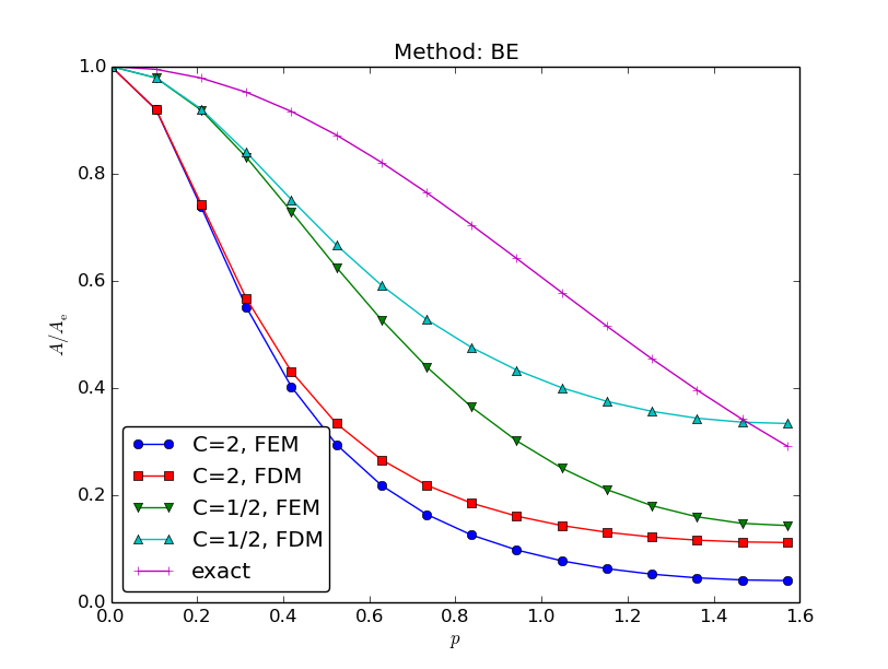
Comparison of coarse-mesh amplification factors for Backward Euler discretization of a 1D diffusion equation

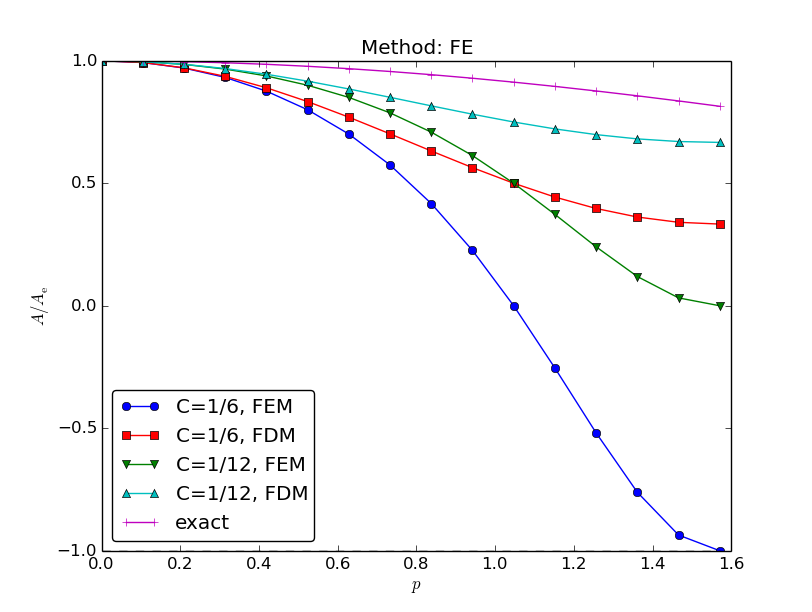
Comparison of fine-mesh amplification factors for Forward Euler discretization of a 1D diffusion equation

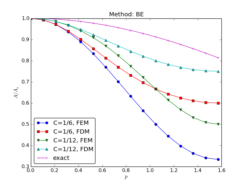
Comparison of fine-mesh amplification factors for Backward Euler discretization of a 1D diffusion equation

Remaining tasks:

• Taylor expansion of the error in the amplification factor \({A_{\small\mbox{e}}} - A\)
• Taylor expansion of the error \(e = ({A_{\small\mbox{e}}}^n - A^n)e^{ikx}\)
• \(L^2\) norm of \(e\)

Exercises

Exercise 1: Analyze a Crank-Nicolson scheme for the diffusion equation

Perform the analysis in the section Analysis of the discrete equations for a 1D diffusion equation \(u_t = {\alpha} u_{xx}\) discretized by the Crank-Nicolson scheme in time:

\[\frac{u^{n+1}- u^n}{\Delta t} = {\alpha} \frac{1}{2}\left( \frac{\partial u^{n+1}}{\partial x^2} + \frac{\partial u^{n}}{\partial x^2}\right),\]

or written compactly with finite difference operators,

\[[D_t u = {\alpha} D_xD_x \overline{u}^t]^{n+\frac{1}{2}}{\thinspace .}\]

(From a strict mathematical point of view, the \(u^n\) and \(u^{n+1}\) in these equations should be replaced by \({u_{\small\mbox{e}}}^n\) and \({u_{\small\mbox{e}}}^{n+1}\) to indicate that the unknown is the exact solution of the PDE discretized in time, but not yet in space, see the section Discretization in time by a Forward Euler scheme.) Make plots similar to those in the section Analysis of the discrete equations. Filename: fe_diffusion.