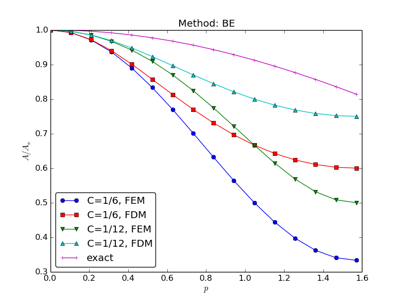
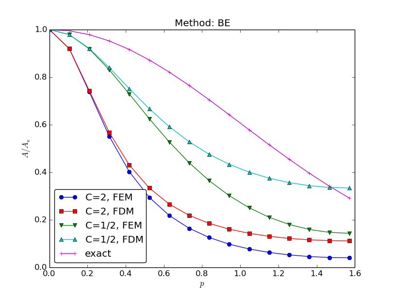
Amplification factor for the Backward Euler method; results
Coarse meshes:
$$
A = \left( 1 + 4C\frac{\sin^2 p}{1 + \frac{2}{3}\sin^2 p}\right)^{-1}
\hbox{ (unconditionally stable)}
$$
$$
\begin{align*}
\frac{\partial u}{\partial t} &= \dfc\nabla^2 u + f(\x, t),\quad
&\x\in\Omega, t\in (0,T]\\
u(\x, 0) & = I(\x),\quad &\x\in\Omega\\
\frac{\partial u}{\partial n} &= 0,\quad &\x\in\partial\Omega,\ t\in (0,T]
\end{align*}
$$
$$
\begin{equation*}
[D_t^+ u = \dfc\nabla^2 u + f]^n,\quad n=1,2,\ldots,N_t-1
\end{equation*}
$$
Solving wrt \( u^{n+1} \):
$$
\begin{equation*}
u^{n+1} = u^n + \Delta t \left( \dfc\nabla^2 u^n + f(\x, t_n)\right)
\end{equation*}
$$
$$
\begin{equation*}
\frac{\partial \uex}{\partial t} = \dfc\nabla^2 \uex + f(\x, t)
\end{equation*}
$$
$$
\begin{equation*}
\uex^{n+1} = \uex^n + \Delta t \left( \dfc\nabla^2 \uex^n + f(\x, t_n)\right)
\end{equation*}
$$
$$
\uex^n \approx u^n = \sum_{j=0}^{N} c_j^{n}\baspsi_j(\x),\quad
\uex^{n+1} \approx u^{n+1} = \sum_{j=0}^{N} c_j^{n+1}\baspsi_j(\x)
$$
$$ R = u^{n+1} - u^n - \Delta t \left( \dfc\nabla^2 u^n + f(\x, t_n)\right)$$
$$ R = u^{n+1} - u^n - \Delta t \left( \dfc\nabla^2 u^n + f(\x, t_n)\right)$$
The weighted residual principle:
$$ \int_\Omega Rw\dx = 0,\quad \forall w\in W$$
results in
$$
\int_\Omega
\left\lbrack
u^{n+1} - u^n - \Delta t \left( \dfc\nabla^2 u^n + f(\x, t_n)\right)
\right\rbrack w \dx =0, \quad \forall w \in W
$$
Galerkin: \( W=V \), \( w=v \)
Isolating the unknown \( u^{n+1} \) on the left-hand side:
$$
\int_{\Omega} u^{n+1}v\dx = \int_{\Omega}
\left\lbrack u^n + \Delta t \left( \dfc\nabla^2 u^n + f(\x, t_n)\right)
\right\rbrack v\dx
$$
Integration by parts of \( \int\dfc(\nabla^2 u^n) v\dx \):
$$ \int_{\Omega}\dfc(\nabla^2 u^n)v \dx =
-\int_{\Omega}\dfc\nabla u^n\cdot\nabla v\dx +
\underbrace{\int_{\partial\Omega}\dfc\frac{\partial u^n}{\partial n}v \dx}_{=0\quad\Leftarrow\quad\partial u^n/\partial n=0}
$$
Variational form:
$$
\begin{equation*}
\int_{\Omega} u^{n+1} v\dx =
\int_{\Omega} u^n v\dx -
\Delta t \int_{\Omega}\dfc\nabla u^n\cdot\nabla v\dx +
\Delta t\int_{\Omega}f^n v\dx,\quad\forall v\in V
\end{equation*}
$$
u: the spatial unknown function to be computedu_1: the spatial function at the previous time level \( t-\Delta t \)u_2: the spatial function at \( t-2\Delta t \)
$$
\begin{equation*}
\int_{\Omega} u v\dx =
\int_{\Omega} u_1 v\dx -
\Delta t \int_{\Omega}\dfc\nabla u_1\cdot\nabla v\dx +
\Delta t\int_{\Omega}f^n v\dx
\end{equation*}
$$
or shorter
$$
\begin{equation*}
(u,v) = (u_1,v) -
\Delta t (\dfc\nabla u_1,\nabla v) +
\Delta t (f^n, v)
\end{equation*}
$$
Insert these in
$$
(u, \baspsi_i) = (u_1,\baspsi_i) -
\Delta t (\dfc\nabla u_1,\nabla\baspsi_i) +
\Delta t (f^n,\baspsi_i)
$$
and order terms as matrix-vector products (\( i=0,\ldots,N \)):
$$
\begin{equation*}
\sum_{j=0}^{N} \underbrace{(\baspsi_i,\baspsi_j)}_{M_{i,j}} c_j =
\sum_{j=0}^{N} \underbrace{(\baspsi_i,\baspsi_j)}_{M_{i,j}} c_{1,j}
-\Delta t \sum_{j=0}^{N}
\underbrace{(\nabla\baspsi_i,\dfc\nabla\baspsi_j)}_{K_{i,j}} c_{1,j}
+ \Delta t (f^n,\baspsi_i)
\end{equation*}
$$
$$
\begin{equation*}
Mc = Mc_1 - \Delta t Kc_1 +\Delta t f
\end{equation*}
$$
$$
\begin{align*}
M &= \{M_{i,j}\},\quad M_{i,j}=(\baspsi_i,\baspsi_j),\quad i,j\in\If\\
K &= \{K_{i,j}\},\quad K_{i,j}=(\nabla\baspsi_i,\dfc\nabla\baspsi_j),\quad i,j\in\If\\
f &= \{(f(\x,t_n),\baspsi_i)\}_{i\in\If}\\
c &= \{c_i\}_{i\in\If}\\
c_1 &= \{c_{1,i}\}_{i\in\If}
\end{align*}
$$
Initial condition:
$$
\begin{align}
\frac{\partial u}{\partial t} &= \dfc\frac{\partial^2 u}{\partial x^2},\quad
&x\in (0,L),\ t\in (0,T],
\tag{1}\\
u(x, 0) & = A\cos(\pi\x/L) + B\cos(10\pi x/L),\quad &x\in[0,L],
\tag{2}\\
\frac{\partial u}{\partial x} &= 0,\quad &x=0,L,\ t\in (0,T]
\tag{3}
\tp
\end{align}
$$
$$ \baspsi_i = \cos(i\pi x/L)\tp$$
\( I(x)\in V \) implies perfect approximation of the initial condition:
$$ c_{1,1}=A,\quad c_{1,10}=B,$$
while \( c_{1,i}=0 \) for \( i\neq 1,10 \).
Note that \( \baspsi_i \) and \( \baspsi_i' \) are orthogonal on \( [0,L] \) such that we only need to compute the diagonal elements \( M_{i,i} \) and \( K_{i,i} \)!
$$ M_{0,0}=L,\quad M_{i,i}=L/2,\ i>0,\quad K_{0,0}=0,\quad K_{i,i}=\frac{\pi^2 i^2}{2L},\ i>0\tp$$
$$
\begin{align*}
Lc_0 &= Lc_{1,0} - \Delta t \cdot 0\cdot c_{1,0},\\
\frac{L}{2}c_i &= \frac{L}{2}c_{1,i} - \Delta t
\frac{\pi^2 i^2}{2L} c_{1,i},\quad i>0\tp
\end{align*}
$$
$$ c_i = (1-\Delta t (\frac{\pi i}{L})^2) c_{1,i}\tp $$
We actually get a closed-form discrete solution:
$$ u^n_i = A(1-\Delta t (\frac{\pi}{L})^2)^n \cos(\pi x/L)
+ B(1-\Delta t (\frac{10\pi }{L})^2)^n \cos(10\pi x/L)\tp$$
Diffusion equation with finite elements is equivalent to
$$
\begin{equation*}
[D_t^+(u + \frac{1}{6}h^2D_xD_x u) = \dfc D_xD_x u + f]^n_i
\end{equation*}
$$
Can lump the mass matrix by Trapezoidal integration and get the standard finite difference scheme
$$
\begin{equation*}
[D_t^+u = \dfc D_xD_x u + f]^n_i
\end{equation*}
$$
Backward Euler scheme in time:
$$
[D_t^- u = \dfc\nabla^2 u + f(\x, t)]^n
$$
$$
\begin{equation*}
\uex^{n} - \Delta t \left( \dfc\nabla^2 \uex^n + f(\x, t_{n})\right) =
\uex^{n-1}
\end{equation*}
$$
$$ \uex^n \approx u^n = \sum_{j=0}^{N} c_j^{n}\baspsi_j(\x),\quad
\uex^{n+1} \approx u^{n+1} = \sum_{j=0}^{N} c_j^{n+1}\baspsi_j(\x)$$
$$
\begin{equation*}
\int_{\Omega} \left( u^{n}v
+ \Delta t \dfc\nabla u^n\cdot\nabla v\right)\dx
= \int_{\Omega} u^{n-1} v\dx +
\Delta t\int_{\Omega}f^n v\dx,\quad\forall v\in V
\end{equation*}
$$
or
$$
\begin{equation*}
(u,v)
+ \Delta t (\dfc\nabla u,\nabla v)
= (u_1,v) +
\Delta t (f^n,v)
\end{equation*}
$$
The linear system: insert \( u=\sum_j c_j\baspsi_i \) and \( u_1=\sum_j c_{1,j}\baspsi_i \),
$$
\begin{equation*}
(M + \Delta t K)c = Mc_1 + \Delta t f
\end{equation*}
$$
Can interpret the resulting equation system as
$$
\begin{equation*}
[D_t^-(u + \frac{1}{6}h^2D_xD_x u) = \dfc D_xD_x u + f]^n_i
\end{equation*}
$$
Lumped mass matrix (by Trapezoidal integration) gives a standard finite difference method:
$$
\begin{equation*}
[D_t^- u = \dfc D_xD_x u + f]^n_i
\end{equation*}
$$
Dirichlet condition at \( x=0 \) and Neumann condition at \( x=L \):
$$
\begin{align*}
u(\x,t) &= u_0(\x,t),\quad & \x\in\partial\Omega_D\\
-\dfc\frac{\partial}{\partial n} u(\x,t) &= g(\x,t),\quad
& \x\in\partial{\Omega}_N
\end{align*}
$$
Forward Euler in time, Galerkin's method, and integration by parts:
$$
\begin{equation*}
\int_\Omega u^{n+1}v\dx =
\int_\Omega (u^n - \Delta t\dfc\nabla u^n\cdot\nabla v)\dx +
\Delta t\int_\Omega fv \dx -
\Delta t\int_{\partial\Omega_N} gv\ds,\quad \forall v\in V
\end{equation*}
$$
Requirement: \( v=0 \) on \( \partial\Omega_D \)
$$ u^n(\x) = u_0(\x,t_n) + \sum_{j\in\If}c_j^n\baspsi_j(\x)$$
$$
\begin{align*}
\sum_{j\in\If} & \left(\int_\Omega \baspsi_i\baspsi_j\dx\right)
c^{n+1}_j = \sum_{j\in\If}
\left(\int_\Omega\left( \baspsi_i\baspsi_j -
\Delta t\dfc\nabla \baspsi_i\cdot\nabla\baspsi_j\right)\dx\right) c_j^n - \\
&\quad \int_\Omega\left( \left(u_0(\x,t_{n+1}) - u_0(\x,t_n)\right) \baspsi_i
+ \Delta t\dfc\nabla u_0(\x,t_n)\cdot\nabla
\baspsi_i\right)\dx \\
& \quad + \Delta t\int_\Omega f\baspsi_i\dx -
\Delta t\int_{\partial\Omega_N} g\baspsi_i\ds,
\quad i\in\If
\end{align*}
$$
$$
\begin{align*}
u^n &= \sum_{j\in\Ifb} U_j^n\basphi_j + \sum_{j\in\If}c_{1,j}\basphi_{\nu(j)},\\
u^{n+1} &= \sum_{j\in\Ifb} U_j^{n+1}\basphi_j +
\sum_{j\in\If}c_{j}\basphi_{\nu(j)}
\end{align*}
$$
$$
\begin{align*}
\sum_{j\in\If} & \left(\int_\Omega \basphi_i\basphi_j\dx\right)
c_j = \sum_{j\in\If}
\left(\int_\Omega\left( \basphi_i\basphi_j -
\Delta t\dfc\nabla \basphi_i\cdot\nabla\basphi_j\right)\dx\right) c_{1,j}
- \\
&\quad \sum_{j\in\Ifb}\int_\Omega\left( \basphi_i\basphi_j(U_j^{n+1} - U_j^n)
+ \Delta t\dfc\nabla \basphi_i\cdot\nabla
\basphi_jU_j^n\right)\dx \\
&\quad + \Delta t\int_\Omega f\basphi_i\dx -
\Delta t\int_{\partial\Omega_N} g\basphi_i\ds,
\quad i\in\If
\end{align*}
$$
$$
\begin{align*}
\sum_{j\in\If}
\biggl(\underbrace{\int_\Omega \basphi_i\basphi_j\dx}_{M_{i,j}}\biggr)
c_j &= \sum_{j\in\If}
\biggl(\underbrace{\int_\Omega \basphi_i\basphi_j \dx}_{M_{i,j}} -
\Delta t\underbrace{\int_\Omega
\dfc\nabla \basphi_i\cdot\nabla\basphi_j\dx}_{K_{i,j}}\biggr) c_{1,j}
\\
&\quad \underbrace{+\Delta t\int_\Omega f\basphi_i\dx -
\Delta t\int_{\partial\Omega_N} g\basphi_i\ds}_{f_i},\quad i\in\If
\end{align*}
$$
$$
\begin{equation*}
Mc = b,\quad b = Mc_1 - \Delta t Kc_1 + \Delta t f
\end{equation*}
$$
For each \( k \) where a Dirichlet condition applies, \( u(\xno{k},t_{n+1})=U_k^{n+1} \),
Or apply the slightly more complicated modification which preserves symmetry of \( M \)
Backward Euler discretization in time gives a more complicated coefficient matrix:
$$
\begin{equation*}
Ac=b,\quad A = M + \Delta t K,\quad b = Mc_1 + \Delta t f
\end{equation*}
$$
Observe: \( A_{k,k} = M_{k,k} + \Delta t K_{k,k} = 1 + 0 \), so \( c_k = U_k^{n+1} \)
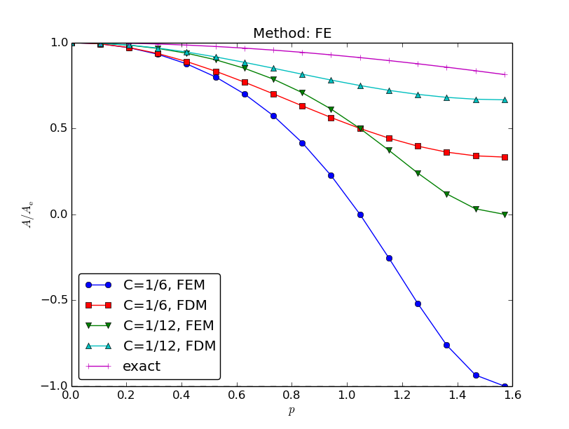
The diffusion equation \( u_t = \dfc u_{xx} \) allows a (Fourier) wave component
$$
\begin{equation*}
u = \Aex^n e^{ikx},\quad \Aex = e^{-\dfc k^2\Delta t}
\end{equation*}
$$
Numerical schemes often allow the similar solution
$$
\begin{equation*}
u^n_q = A^n e^{ikx}
\end{equation*}
$$
$$
\begin{align*}
[D_t^+ A^n e^{ikq\Delta x}]^n &= A^n e^{ikq\Delta x}\frac{A-1}{\Delta t},\\
[D_t^- A^n e^{ikq\Delta x}]^n &= A^n e^{ikq\Delta x}\frac{1-A^{-1}}{\Delta t},\\
[D_t A^n e^{ikq\Delta x}]^{n+\half} &= A^{n+\half} e^{ikq\Delta x}\frac{A^{\half}-A^{-\half}}{\Delta t} = A^ne^{ikq\Delta x}\frac{A-1}{\Delta t},\\
[D_xD_x A^ne^{ikq\Delta x}]_q &= -A^n \frac{4}{\Delta x^2}\sin^2\left(\frac{k\Delta x}{2}\right)
\end{align*}
$$
Introduce \( p=k\Delta x/2 \) and \( C=\dfc\Delta t/\Delta x^2 \):
$$ A = 1 - 4C\frac{\sin^2 p}{1 - \underbrace{\frac{2}{3}\sin^2 p}_{\hbox{from }M}}$$
(See notes for details)
Stability: \( |A|\leq 1 \):
$$
\begin{equation*}
C\leq \frac{1}{6}\quad\Rightarrow\quad \Delta t\leq \frac{\Delta x^2}{6\dfc}
\end{equation*}
$$
Finite differences: \( C\leq {\half} \), so finite elements give a stricter stability criterion for this PDE!
Coarse meshes:
$$
A = \left( 1 + 4C\frac{\sin^2 p}{1 + \frac{2}{3}\sin^2 p}\right)^{-1}
\hbox{ (unconditionally stable)}
$$