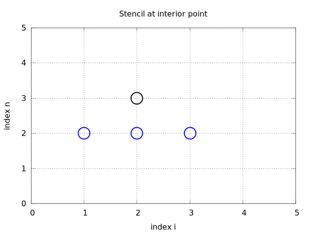
The discrete solution
- The numerical solution is a mesh function: \( u_i^n \approx \uex(x_i,t_n) \)
- Finite difference stencil (or scheme): equation for \( u^n_i \) involving neighboring space-time points
The famous diffusion equation, also known as the heat equation, reads
$$ \frac{\partial u}{\partial t} =
\dfc \frac{\partial^2 u}{\partial x^2}
$$
Here,
Alternative, compact notation:
$$ u_t = \dfc u_{xx} $$
$$
\begin{align}
\frac{\partial u}{\partial t} &=
\dfc \frac{\partial^2 u}{\partial x^2}, \quad x\in (0,L),\ t\in (0,T]
\tag{1}\\
u(x,0) &= I(x), \quad x\in [0,L]
\tag{2}\\
u(0,t) & = 0, \quad t>0,
\tag{3}\\
u(L,t) & = 0, \quad t>0\tp
\tag{4}
\end{align}
$$
Note:
Mesh in time:
$$
\begin{equation}
0 = t_0 < t_1 < t_2 < \cdots < t_{N_t-1} < t_{N_t} = T \tag{5}
\end{equation}
$$
Mesh in space:
$$
\begin{equation}
0 = x_0 < x_1 < x_2 < \cdots < x_{N_x-1} < x_{N_x} = L \tag{6}
\end{equation}
$$
Uniform mesh with constant mesh spacings \( \Delta t \) and \( \Delta x \):
$$
\begin{equation}
x_i = i\Delta x,\ i=0,\ldots,N_x,\quad
t_i = n\Delta t,\ n=0,\ldots,N_t
\tag{7}
\end{equation}
$$
Require the PDE (1) to be fulfilled at an arbitrary interior mesh point \( (x_i,t_n) \) leads to
$$
\begin{equation}
\frac{\partial}{\partial t} u(x_i, t_n) =
\dfc\frac{\partial^2}{\partial x^2} u(x_i, t_n)
\tag{8}
\end{equation}
$$
Applies to all interior mesh points: \( i=1,\ldots,N_x-1 \) and \( n=1,\ldots,N_t-1 \)
For \( n=0 \) we have the initial conditions \( u=I(x) \) and \( u_t=0 \)
At the boundaries \( i=0,N_x \) we have the boundary condition \( u=0 \).
Use a forward difference in time and a centered difference in space (Forward Euler scheme):
$$
\begin{equation}
[D_t^+ u = \dfc D_xD_x u]^n_i
\tag{9}
\end{equation}
$$
Written out,
$$
\begin{equation}
\frac{u^{n+1}_i-u^n_i}{\Delta t} = \dfc \frac{u^{n}_{i+1} - 2u^n_i + u^n_{i-1}}{\Delta x^2}
\tag{10}
\end{equation}
$$
Initial condition: \( u^0_i = I(x_i) \), \( i=0,1,\ldots,N_x \).
Solve the discretized PDE for the unknown \( u^{n+1}_i \):
$$
\begin{equation}
u^{n+1}_i = u^n_i + F\left(
u^{n}_{i+1} - 2u^n_i + u^n_{i-1}\right)
\tag{11}
\end{equation}
$$
where
$$ F = \dfc\frac{\Delta t}{\Delta x^2} $$
$$ F = \dfc\frac{\Delta t}{\Delta x^2} $$
There is only one parameter, \( F \), in the discrete model: \( F \) lumps mesh parameters \( \Delta t \) and \( \Delta x \) with the only physical parameter, the diffusion coefficient \( \dfc \). The value \( F \) and the smoothness of \( I(x) \) govern the quality of the numerical solution.
We visit one mesh point \( (x_i,t_{n+1}) \) at a time, and we have an explicit formula for computing the associated \( u^{n+1}_i \) value. The spatial points can be updated in any sequence, but the time levels \( t_n \) must be updated in cronological order: \( t_n \) before \( t_{n+1} \).
x = linspace(0, L, Nx+1)    # mesh points in space
dx = x[1] - x[0]
t = linspace(0, T, Nt+1)    # mesh points in time
dt = t[1] - t[0]
F = a*dt/dx**2
u   = zeros(Nx+1)
u_1 = zeros(Nx+1)

# Set initial condition u(x,0) = I(x)
for i in range(0, Nx+1):
    u_1[i] = I(x[i])

for n in range(0, Nt):
    # Compute u at inner mesh points
    for i in range(1, Nx):
        u[i] = u_1[i] + F*(u_1[i-1] - 2*u_1[i] + u_1[i+1])

    # Insert boundary conditions
    u[0] = 0;  u[Nx] = 0

    # Update u_1 before next step
    u_1[:]= u
    # or more efficient switch of references
    #u_1, u = u, u_1
web page or a movie file.
tmp_frame%04d.png filestmp_frame0000.png, tmp_frame0001.png, ...How to make movie file in modern formats:
Terminal> name=tmp_frame%04d.png
Terminal> fps=8  # frames per second in movie
Terminal> avconv -r $fps -i $name -vcodec flv       movie.flv
Terminal> avconv -r $fps -i $name -vcodec libx64    movie.mp4
Terminal> avconv -r $fps -i $name -vcodec libvpx    movie.webm
Terminal> avconv -r $fps -i $name -vcodec libtheora movie.ogg
\( N_x=50 \). The method results in a growing, unstable solution if \( F>0.5 \).
|
Choosing \( F=0.5 \) gives a strange saw tooth-like curve.
|
Lowering \( F \) to 0.25 gives a smooth (expected) solution.
|
\( N_x=50 \). \( F=0.5 \).
|
|
|
Backward difference in time, centered difference in space:
$$
\begin{equation}
[D_t^- u = D_xD_x u]^n_i
\tag{12}
\end{equation}
$$
Written out:
$$
\begin{equation}
\frac{u^{n}_i-u^{n-1}_i}{\Delta t} = \dfc\frac{u^{n}_{i+1} - 2u^n_i + u^n_{i-1}}{\Delta x^2}
\tag{13}
\end{equation}
$$
Assumption: \( u^{n-1}_i \) is computed, but all quantities at the new time level \( t_n \) are unknown.
We cannot solve wrt \( u^n_i \) because that unknown value is coupled to two other unknown values: \( u^n_{i-1} \) and \( u^n_{i+1} \). That is, all the new unknown values are coupled to each other in a linear system of algebraic equations.
Equation (13) written for \( i=1,\ldots,Nx-1= 1,2 \) becomes
$$
\begin{align}
\frac{u^{n}_1-u^{n-1}_1}{\Delta t} &= \dfc\frac{u^{n}_{2} - 2u^n_1 + u^n_{0}}{\Delta x^2}
\tag{14}\\
\frac{u^{n}_2-u^{n-1}_2}{\Delta t} &= \dfc\frac{u^{n}_{3} - 2u^n_2 + u^n_{1}}{\Delta x^2}
\tag{15}
\end{align}
$$
(The boundary values \( u^n_0 \) and \( u^n_3 \) are known as zero.)
Collecting the unknown new values on the left-hand side and writing as \( 2\times 2 \) matrix system:
$$ \left(\begin{array}{cc}
1+ 2F & - F\\
- F & 1+ 2F
\end{array}\right)
\left(\begin{array}{c}
u^{n}_1\\
u^{n}_{2}\\
\end{array}\right)
=
\left(\begin{array}{c}
u^{n-1}_1\\
u^{n-1}_2
\end{array}\right)
$$
Discretization methods that lead linear systems are known as implicit methods.
Discretization methods that avoid linear systems and have an explicit formula for each new value of the unknown are called explicit methods.
$$
\begin{equation}
- F_o u^n_{i-1} + \left(1+ 2F_o \right) u^{n}_i - F_o u^n_{i+1} =
u_{i-1}^{n-1}
\tag{16}
\end{equation}
$$
for \( i=1,\ldots,Nx-1 \).
What are the unknowns in the linear system?
The linear system in matrix notation:
$$
\begin{equation*} AU = b,\quad U=(u^n_0,\ldots,u^n_{N_x})
\end{equation*}
$$
$$
\begin{equation}
A =
\left(
\begin{array}{cccccccccc}
A_{0,0} & A_{0,1} & 0
&\cdots &
\cdots & \cdots & \cdots &
\cdots & 0 \\
A_{1,0} & A_{1,1} & 0 & \ddots & & & & & \vdots \\
0 & A_{2,1} & A_{2,2} & A_{2,3} &
\ddots & & & & \vdots \\
\vdots & \ddots & & \ddots & \ddots & 0 & & & \vdots \\
\vdots & & \ddots & \ddots & \ddots & \ddots & \ddots & & \vdots \\
\vdots & & & 0 & A_{i,i-1} & A_{i,i} & A_{i,i+1} & \ddots & \vdots \\
\vdots & & & & \ddots & \ddots & \ddots &\ddots & 0 \\
\vdots & & & & &\ddots & \ddots &\ddots & A_{N_x-1,N_x} \\
0 &\cdots & \cdots &\cdots & \cdots & \cdots & 0 & A_{N_x,N_x-1} & A_{N_x,N_x}
\end{array}
\right)
\tag{17}
\end{equation}
$$
The nonzero elements are given by
$$
\begin{align}
A_{i,i-1} &= -F_o
\tag{18}\\
A_{i,i} &= 1+ 2F_o
\tag{19}\\
A_{i,i+1} &= -F_o
\tag{20}
\end{align}
$$
for \( i=1,\ldots,N_x-1 \).
The equations for the boundary points correspond to
$$
A_{0,0} = 1,\quad A_{0,1} = 0,\quad A_{N_x,N_x-1} = 0,\quad
A_{N_x,N_x} = 1
$$
$$
\begin{equation}
b = \left(\begin{array}{c}
b_0\\
b_1\\
\vdots\\
b_i\\
\vdots\\
b_{N_x}
\end{array}\right)
\tag{21}
\end{equation}
$$
with
$$
\begin{align}
b_0 &= 0
\tag{22}\\
b_i &= u^{n-1}_i,\quad i=1,\ldots,N_x-1
\tag{23}\\
b_{N_x} &= 0
\tag{24}
\end{align}
$$
x = linspace(0, L, Nx+1)   # mesh points in space
dx = x[1] - x[0]
t = linspace(0, T, N+1)    # mesh points in time
u   = zeros(Nx+1)
u_1 = zeros(Nx+1)

# Data structures for the linear system
A = zeros((Nx+1, Nx+1))
b = zeros(Nx+1)

for i in range(1, Nx):
    A[i,i-1] = -F
    A[i,i+1] = -F
    A[i,i] = 1 + 2*F
A[0,0] = A[Nx,Nx] = 1

# Set initial condition u(x,0) = I(x)
for i in range(0, Nx+1):
    u_1[i] = I(x[i])

import scipy.linalg

for n in range(0, Nt):
    # Compute b and solve linear system
    for i in range(1, Nx):
        b[i] = -u_1[i]
    b[0] = b[Nx] = 0
    u[:] = scipy.linalg.solve(A, b)

    # Update u_1 before next step
    u_1, u = u, u_1
scipy.sparse enables storage and calculations with the three
nonzero diagonals only
# Representation of sparse matrix and right-hand side
diagonal  = zeros(Nx+1)
lower     = zeros(Nx)
upper     = zeros(Nx)
b         = zeros(Nx+1)
# Precompute sparse matrix
diagonal[:] = 1 + 2*F
lower[:] = -F  #1
upper[:] = -F  #1
# Insert boundary conditions
diagonal[0] = 1
upper[0] = 0
diagonal[Nx] = 1
lower[-1] = 0

import scipy.sparse
A = scipy.sparse.diags(
    diagonals=[main, lower, upper],
    offsets=[0, -1, 1], shape=(Nx+1, Nx+1),
    format='csr')

# Set initial condition
for i in range(0,Nx+1):
    u_1[i] = I(x[i])

for n in range(0, Nt):
    b = u_1
    b[0] = b[-1] = 0.0  # boundary conditions
    u[:] = scipy.sparse.linalg.spsolve(A, b)
    # Switch variables before next step
    u_1, u = u, u_1
\( N_x=50 \). \( F=0.5 \).
\( N_x=50 \).
|
\( F=0.5 \).
|
\( F=5 \).
|
The PDE is sampled at points \( (x_i,t_{n+\half}) \) (at the spatial mesh points, but in between two temporal mesh points).
$$
\frac{\partial}{\partial t} u(x_i, t_{n+\half}) =
\dfc\frac{\partial^2}{\partial x^2}u(x_i, t_{n+\half})
$$
for \( i=1,\ldots,N_x-1 \) and \( n=0,\ldots, N_t-1 \).
Centered differences in space and time:
$$ [D_t u = \dfc D_xD_x u]^{n+\half}_i$$
Right-hand side term:
$$ \frac{1}{\Delta x^2}\left(u^{n+\half}_{i-1} - 2u^{n+\half}_i + u^{n+\half}_{i+1}\right)$$
Problem: \( u^{n+\half}_i \) is not one of the unknowns we compute.
Solution: replace \( u^{n+\half}_i \) by an arithmetic average:
$$ u^{n+\half}_i\approx
\half\left(u^{n}_i +u^{n+1}_{i}\right)
$$
In compact notation (arithmetic average in time \( \overline{u}^t \)):
$$ [D_t u = \dfc D_xD_x \overline{u}^t]^{n+\half}_i$$
$$
\begin{equation}
u^{n+1}_i - \half F(u^{n+1}_{i-1} - 2u^{n+1}_i + u^{n+1}_{i+1})
= u^{n}_i + \half F(u^{n}_{i-1} - 2u^{n}_i + u^{n}_{i+1})
\tag{25}
\end{equation}
$$
Observe:
Now,
$$
\begin{align}
A_{i,i-1} &= -\half F_o
\tag{26}\\
A_{i,i} &= \half + F_o
\tag{27}\\
A_{i,i+1} &= -\half F_o
\tag{28}
\end{align}
$$
for internal points. For boundary points,
$$
\begin{align}
A_{0,0} &= 1
\tag{29}\\
A_{0,1} &= 0
\tag{30}\\
A_{N_x,N_x-1} &= 0
\tag{31}\\
A_{N_x,N_x} &= 1
\tag{32}
\end{align}
$$
Right-hand side:
$$
\begin{align}
b_0 &= 0
\tag{33}\\
b_i &= u^{n-1}_i,\quad i=1,\ldots,N_x-1
\tag{34}\\
b_{N_x} &= 0 \tag{35}
\end{align}
$$
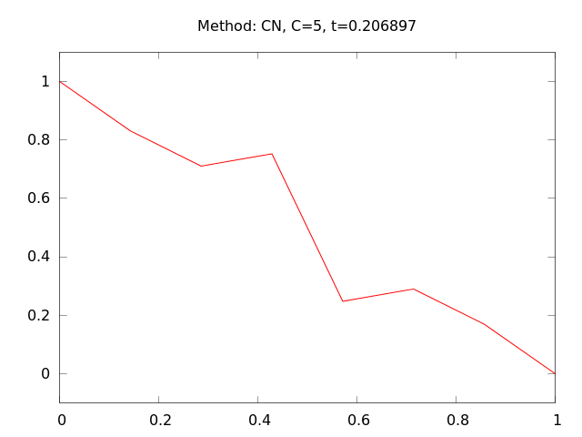
Crank-Nicolson never blows up, so any \( F \) can be used (modulo loss of accuracy).
|
\( N_x=50 \).
\( F=5 \) gives instabilities.
|
\( N_x=50 \).
\( F=0.5 \) gives a smooth solution.
|
\( N_x=50 \).
|
\( F=0.5 \).
|
\( F=5 \).
|
The \( \theta \) rule condenses a family of finite difference approximations in time to one formula
Applied to \( u_t=\dfc u_{xx} \):
$$ \frac{u^{n+1}_i-u^n_i}{\Delta t} =
\dfc\left( \theta \frac{u^{n+1}_{i+1} - 2u^{n+1}_i + u^{n+1}_{i-1}}{\Delta x^2}
+ (1-\theta) \frac{u^{n}_{i+1} - 2u^n_i + u^n_{i-1}}{\Delta x^2}\right)
$$
Matrix entries:
$$ A_{i,i-1} = -F_o\theta,\quad A_{i,i} = 1+2F_o\theta\quad,
A_{i,i+1} = -F_o\theta$$
Right-hand side:
$$ b_i = u^n_{i} + F_o(1-\theta)
\frac{u^{n}_{i+1} - 2u^n_i + u^n_{i-1}}{\Delta x^2}
$$
Laplace equation:
$$ \nabla^2 u = 0,\quad \mbox{1D: } u''(x)=0$$
Poisson equation:
$$ -\nabla^2 u = f,\quad \mbox{1D: } -u''(x)=f(x)$$
These are limiting behavior of time-dependent diffusion equations if
$$ \lim_{t\rightarrow\infty}\frac{\partial u}{\partial t} = 0$$
Then \( u_t = \dfc u_{xx} + 0 \) in the limit \( t\rightarrow\infty \) reduces to
$$ u_{xx} + f = 0$$
Looking at the numerical schemes, \( F\rightarrow\infty \) leads to the Laplace or Poisson equations (without \( f \) or with \( f \), resp.).
Good news: choose \( F \) large in the BE or CN schemes and one time step is enough to produce the stationary solution for \( t\rightarrow\infty \).
These extensions are performed exactly as for a wave equation as they only affect the spatial derivatives (which are the same as in the wave equation).
Future versions of this document will for completeness and independence of the wave equation document feature info on the three points. The Robin condition is new, but straightforward to handle:
$$ -\dfc\frac{\partial u}{\partial n} = h_T(u-U_s),\quad
[-\dfc D_x u = h_T(u-U_s)]^n_i
$$
The PDE
$$
u_t = \dfc u_{xx}
$$
admits solutions
$$
u(x,t) = Qe^{-\dfc k^2 t}\sin\left( kx\right)
$$
Observations from this solution:
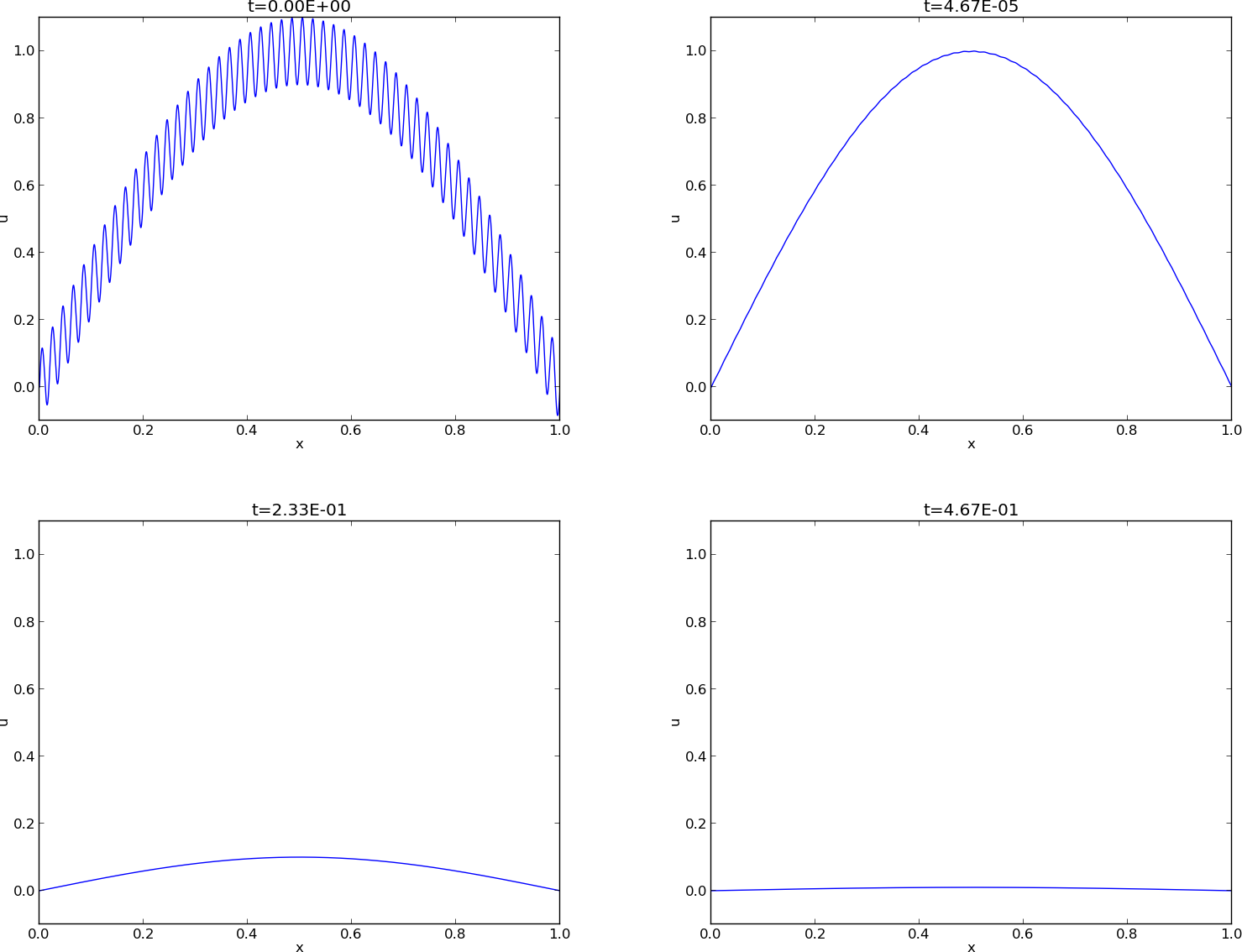
Test problem:
$$
\begin{align*}
u_t &= u_{xx},\quad &x\in (0,1),\ t\in (0,T]\\
u(0,t) &= u(1,t) = 0,\quad &t\in (0,T]\\
u(x,0) & = \sin (\pi x) + 0.1\sin(100\pi x)
\end{align*}
$$
Exact solution:
$$
u(x,t) = e^{-\pi^2 t}\sin (\pi x) + 0.1e^{-\pi^2 10^4 t}\sin (100\pi x)
$$
Two pieces of a material, at different temperatures, are brought in contact at \( t=0 \). Assume the end points of the pieces are kept at the initial temperature. How does the heat flow from the hot to the cold piece?
Or: A huge ion concentration on one side of a synapse in the brain (concentration discontinuity) is released and ions move by diffusion.
Assume a 1D model is sufficient (e.g., insulated rod):
$$
u(x,0)=\left\lbrace
\begin{array}{ll}
U_L, & x < L/2\\
U_R,& x\geq L/2
\end{array}\right.
$$
$$ \frac{\partial u}{\partial t} = \dfc
\frac{\partial^2 u}{\partial x^2},\quad u(0,t)=U_L,\ u(L,t)=U_R$$
Discrete model:
$$ [D_t^- u = \dfc D_xD_x]^n_i $$
results in a (tridiagonal) linear system
$$
- F u^n_{i-1} + \left(1+ 2F \right) u^{n}_i - F u^n_{i+1} =
u_{i-1}^{n-1}
$$
where
$$ F = \dfc\frac{\Delta t}{\Delta x^2} $$
is the mesh Fourier number
Discrete model:
$$ [D_t^+ u = \dfc D_xD_x]^n_i $$
results in the explicit updating formula
$$ u^{n+1}_i = u^n_i + F\left(
u^{n}_{i+1} - 2u^n_i + u^n_{i-1}\right)
$$
Discrete model:
$$ [D_t u = \dfc D_xD_x\overline{u}^t]^n_i $$
results in a tridiagonal linear system
Represent \( I(x) \) as a Fourier series
$$
I(x) \approx \sum_{k\in K} b_k e^{ikx}
$$
The corresponding sum for \( u \) is
$$
u(x,t) \approx \sum_{k\in K} b_k e^{-\dfc k^2t}e^{ikx}
$$
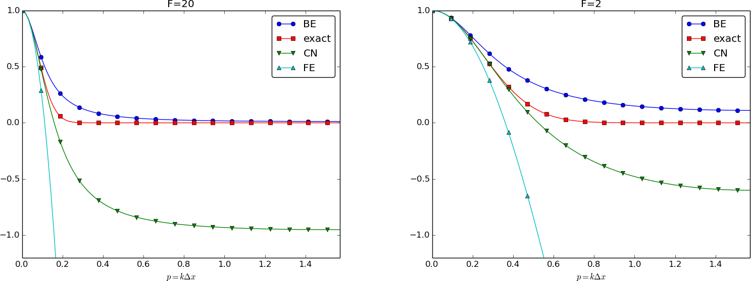
Such solutions are also accepted by the numerical schemes, but with an amplification factor \( A \) different from \( \exp{({-\dfc k^2t})} \):
$$
u^n_q = A^n e^{ikq\Delta x} = A^ne^{ikx}
$$
Stability:
Accuracy:
$$
\begin{equation*} [D_t^+ u = \dfc D_xD_x u]^n_q \end{equation*}
$$
Inserting
$$ u^n_q = A^n e^{ikq\Delta x}$$
leads to
$$
A = 1 -4F\sin^2\left(
\frac{k\Delta x}{2}\right),\quad
F = \frac{\dfc\Delta t}{\Delta x^2}\mbox{ (mesh Fourier number)}
$$
The complete numerical solution is
$$
u^n_q = (1 -4F\sin^2 p)^ne^{ikq\Delta x},\quad
p = k\Delta x/2
$$
Key spatial discretization quantity: the dimensionless \( p=\half k\Delta x \)
We always have \( A\leq 1 \). The condition \( A\geq -1 \) implies
$$ 4F\sin^2p\leq 2 $$
The worst case is when \( \sin^2 p=1 \), so a sufficient criterion for
stability is
$$ F\leq {\half} $$
or:
$$ \Delta t\leq \frac{\Delta x^2}{2\dfc} $$
Less favorable criterion than for \( u_{tt}=c^2u_{xx} \): halving \( \Delta x \) implies time step \( \frac{1}{4}\Delta t \) (not just \( \half\Delta t \) as in a wave equation). Need very small time steps for fine spatial meshes!
$$
\begin{equation*} [D_t^- u = \dfc D_xD_x u]^n_q\end{equation*}
$$
$$ u^n_q = A^n e^{ikq\Delta x}$$
$$ A = (1 + 4F\sin^2p)^{-1} $$
$$ u^n_q = (1 + 4F\sin^2p)^{-n}e^{ikq\Delta x} $$
Stability: We see that \( |A| < 1 \) for all \( \Delta t>0 \) and that \( A>0 \) (no oscillations)
The scheme
$$ [D_t u = \dfc D_xD_x \overline{u}^x]^{n+\half}_q$$
leads to
$$ A = \frac{ 1 - 2F\sin^2p}{1 + 2F\sin^2p} $$
$$ u^n_q = \left(\frac{ 1 - 2F\sin^2p}{1 + 2F\sin^2p}\right)^ne^{ikp\Delta x}$$
Stability: The criteria \( A>-1 \) and \( A < 1 \) are fulfilled for any \( \Delta t >0 \)
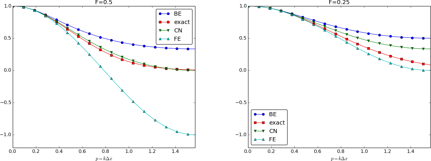
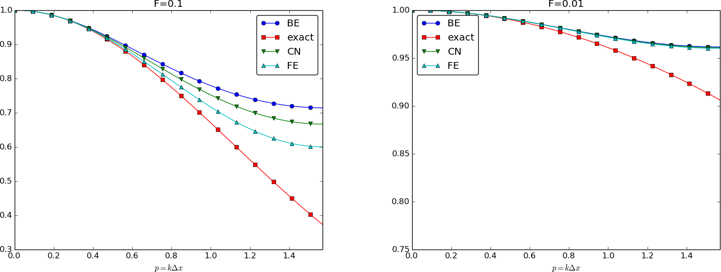
$$
\begin{align*}
\Aex &= \exp{(-\alpha k^2\Delta t)} = \exp{(-4Fp^2)}\\
A &= 1 -4F\sin^2\left(\frac{k\Delta x}{2}\right)\quad\mbox{Forward Euler}\\
A &= (1 + 4F\sin^2p)^{-1}\quad\mbox{Backward Euler}\\
A &= \frac{ 1 - 2F\sin^2p}{1 + 2F\sin^2p}\quad\mbox{Crank-Nicolson}
\end{align*}
$$
Note: \( \Aex = \exp{(-\dfc k^2\Delta t)}=\exp{(-F k^2\Delta x^2)}= \exp{(-F4p^2)} \).
The problems of correct damping for \( u_t = u_{xx} \) is partially manifested in the similar time discretization schemes for \( u'(t)=-\dfc u(t) \).