Introduction
FEniCS solver with boundary conditions in Fortran
The FEniCS solver
The Fortran code for modeling boundary conditions
Coupling the Python FEniCS solver with the Fortran routine
FEniCS solver with optimization in Octave
Basic use of Pytave
Calling the MATLAB/Octave software
The FEniCS PDE solver
Coupling FEniCS and the MATLAB/Octave software
Installing Pytave
How to interface a C++/DOLFIN code from Python
The C++ class
Compiling and linking at the Python DOLFIN level
Compiling and linking at the Instant level
FEniCS solver coupled with ODE solver in C++
Wrapping with F2PY
C API to C++ code
Writing corresponding Fortran signatures
Building the extension module
Main program in Python
A pure C version of the C++ class
Wrapping with SWIG
Wrapping with Cython
Acknowledgment
References
FEniCS is an easy-to-use tool for solving partial differential equations (PDEs) and enables very flexible specifications of PDE problems. However, many scientific problems require (much) more than solving PDEs, and in those cases a FEniCS solver must be coupled to other types of software. This is usually easy and convenient if the FEniCS solver is coded in Python and the other software is either written in Python or easily accessible from Python.
Coupling of FEniCS solvers in Python with MATLAB, Fortran, C, or C++ codes is possible, and in principle straightforward, but there might be a lot of technical details in practice. Many potential FEniCS users already have substantial pieces of software in other more traditional scientific computing languages, and the new solvers they write in FEniCS may need to communicate with this existing and well-tested software. Unfortunately, the world of gluing computer code in very different languages with the aid of tools like F2PY, SWIG, Cython, and Instant is seldom the focal point of a computational scientist. We have therefore written this document to provide some examples and associated detailed explanations on how the mentioned tools can be used to combine FEniCS solvers in Python with other code written in MATLAB, Fortran, C, and C++. We believe that even if the examples are short and limited in complexity, the couplings are technically complicated and broad enough to cover a range of different situations in the real world.
To illustrate the tools and techniques, we focus on four specific case studies:
The present tutorial is found on GitHub: https://github.com/hplgit/fenics-mixed. The following command downloads all the files:
Terminal> git clone https://github.com/hplgit/fenics-mixed.git
The source code for the examples are located in the subdirectory doc/src/src-fenics-mixed. The code examples are tested with FEniCS version 1.2.
Fortran programs are usually easy to interface in Python by using the wrapper code generator F2PY. F2PY supports Fortran 77, Fortran 90, and even C (and thereby C++, see the section FEniCS solver coupled with ODE solver in C++). It is our experience that F2PY is much more straightforward to use than the other tools we describe for interfacing Python with compiled languages. F2PY is therefore a natural starting point for our examples.
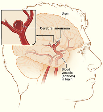
The present worked example involves solving the Navier-Stokes equations by a FEniCS solver, but calling up a Fortran 77 code for modeling the boundary conditions. The physical problem concerns blood flow in a cerebral aneurysm. An aneurysm is a balloon-shaped deformation of a cerebral artery, see Figure 1. Some aneurysms rupture and cause stroke, while other remain stable for long periods of time, and it is currently not possible to determine the rupture risk in a patient-specific manner. Computational studies have recently demonstrated that fluid dynamics simulations can be used to discriminate ruptured from non-ruptured aneurysms [4] [5] [6] [7], retrospectively, and have therefore demonstrated the potential of simulations to many clinicians.
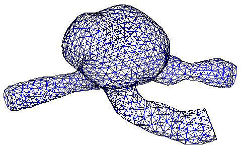
Figure 2: A DOLFIN mesh illustrating a patient-specific aneurysm geometry.
To model blood flow we assume that blood is Newtonian and incompressible with a viscosity of 0.0035 Pa s and density similar to water. The equations read
$$ \begin{align} \rho (\frac{ \partial v}{\partial t} + (v \cdot \nabla) v) &= -\nabla p + \mu \Delta v + f & \mbox{ in }\Omega \\ \nabla \cdot v &= 0 & \mbox{ in } \Omega \end{align} $$ Here, \( v \) and \( p \) are the unknown blood velocity and pressure, respectively, while \( \mu \) is the viscosity and \( \rho \) the density.
Quite often the outlet boundary conditions are unknown. It is therefore common to model the boundary conditions using differential equations of lower dimension. In our case, we assume that the pressure at the inlet or outlet boundaries can be modeled by a system of ODEs:
$$ \begin{align} \frac{\partial P_i}{\partial t} &= f(P_i, v, p, \ldots) & \mbox{ on } \partial \Omega_o . \end{align} $$ These ODEs are coupled to the Navier-Stokes equations through the inlet or outlet boundary condition
$$ \begin{align} \mu \frac{\partial v}{\partial n} + p n &= P_o & \mbox{ on } \partial \Omega_o \end{align} $$
The Navier-Stokes solver is implemented in FEniCS as a
class NSSolver.
The typical usage of the class goes as follows:
   solver = NSSolver()
   solver.setIC()
   t = 0
   dt = 0.01
   T = 1.0
   P1, P2 = 0, 0
   while t < T:
       t += dt
       solver.advance_one_time_step((P1, P2), t)
The setIC() function sets the initial conditions. Futhermore,
P1 and P2 are the pressures at the two outlets at time t.
The implementation details of class NSSolver are not essential to
this document, so we just refer the reader to the relatively short
NSSolver.py file.
The NSSolver class sets Dirichlet condition for the pressure on
inlet and outlet boundaries in terms of prescribed constants in a list
P (one for each prescribed outlet or inlet). Our aim now is to use a
lower-dimensional flow model for computing the Dirichlet values in P
based on physics and the current velocity and pressure fields. One
such model is formulated in terms of ODEs. For an outlet boundary, let
\( P \) be the pressure at the boundary. Then the model for \( P \) is
$$ C \frac{\partial P} {\partial t} = Q - P / R_d, $$ where
$$ Q = \int_{\partial \Omega_o} v \cdot n ds $$ is the volume flux through the boundary \( \partial\Omega_o \) (easily computed in the FEniCS solver). The parameters \( C \) and \( R_d \) must be prescribed along with the initial value of \( P \).
The differential equation for \( P \) can be discretized by a very simple Forward Euler scheme. With \( i \) denoting the time level corresponding to small time steps \( \delta t \) in the fluid solver time step \( \Delta t \), we can write
$$ P^{i+1} = P^i + \delta t (Q - P/R_d)/C,$$ for \( i=0,\ldots, N-1 \), where \( \Delta t = N\delta t \), and then the new pressure outlet condition is \( P=P^{N} \) for the next time step. \( P^0 \) is taken as \( P \) at time \( t \) (\( P \) is the outlet pressure value at time \( t+\Delta t \)).
The computational model for \( P \) is implemented in Fortran. (Our specific model is a simple one; the problem setting is that another research group is continuously developing such models, and their software is in Fortran.) The solver in Fortran is implemented in a file PMODEL.f with the content
      SUBROUTINE PMODEL(P, P_1, R_D, Q, C, N, T)
C     Integrate P in N steps from 0 to T, given start value P_1
      INTEGER N
      REAL*8 P(0:N), P_1, R_D, Q, C, T
      REAL*8 DT
      INTEGER I
Cf2py intent(in) P0, R, Q, C, N
Cf2py intent(out) P

      DT = T/N
      P(0) = P_1
      DO I = 0, N-1
        P(i+1) = P(i) + DT*(Q - P(i)/R_D)/C
      END DO
      END SUBROUTINE PMODEL
Given P_1 as the value of P at time t, the subroutine computes
\( P \) at all the N local time steps (of length DT) up to time t+T,
with P(N) as the final value at that time. We shall call PMODEL
at every time step in the flow solver and let T correspond to the
fluid solver time step \( \Delta t \).
The subroutine is plain Fortran 77 except for some special comment
lines starting with CF2PY. These are needed because in
Fortran, subroutine arguments are both input and output,
but in Python one normally takes all input as arguments to a function
and returns all output arguments. This is technically not
possible in Fortran (or C or C++). With the CF2PY comment lines
we can help the F2PY translater to make the Fortran subroutine look
more "Pythonic" from the Python side. To this end, we need to specify
what arguments that are input and output. All arguments are
input by default, but here we still list them to have complete
specification of every argument in this function. The output
argument, to be returned to Python, must be specified, here P.
Creating a shared library of the Fortran code that we can call from Python as an ordinary module is easy:
Terminal> F2PY -c -m bcmodelf77 ../PMODEL.f
Here, -m bcmodelf77 tells F2PY that the module name is
be bcmodelf77, the -c instructs F2PY to compile and create
a shared library bcmodelf77.so, and PMODEL.f is the name of
the Fortran file to analyze and compile. Our convention is to
compile F2PY modules in a subdirectory of the Fortran code,
which explains why the file here has name ../PMODEL.f.
A little test code can compare the Fortran ODE solver with a couple of manual lines in Python:
import nose.tools as nt

def test_bcmodelf77():
    import bcmodelf77
    C = 0.127
    R_d = 5.43
    N = 2
    P_1 = 16000
    Q = 1000
    T = 0.01
    P_ = bcmodelf77.pmodel(P_1, R_d, Q, C, N, T)

    # Manual formula:
    P1_ = P_1 + T/2*(Q - P_1/R_d)/C
    P1_ = P1_ + T/2*(Q - P1_/R_d)/C
    nt.assert_almost_equal(
        P_[-1], P1_, places=10, msg='F77: %g, manual coding: %s' %
        (P_[-1], P1_))

if __name__ == '__main__':
    test_bcmodelf77()
Note that F2PY turns all upper case letters into lower case when
viewed from Python. Also note that this test function is created as a
nose unit test. Running nosetests in that directory finds all
test_* functions in all files and executes these functions.
Instead of calling the Fortran function directly with many parameters,
we wrap a class around the function such that the syntax of each call
to compute \( P \) becomes simpler. The idea is to let parameters that are
constant through the fluid flow simulation be attributes in the class
so that it is sufficient to provide the varying parameters in the call
to PMODEL. The Python code hopefully
explains this idea clearly:
class BCModel:
    def __init__(self, C, R_d, N, T):
        self.C, self.R, self.N, self.T = C, R_d, N, T

    def __call__(self, P, Q):
        P_ = bcmodelf77.pmodel(
             P, self.R, Q, self.C, self.N, self.T)
        return P_
We can now set all constant parameters at once,
pmodel = BCModel(C=0.127, R_d=5.43, N=2, T=0.01)
and there after call the Fortran subroutine PMODEL by
pmodel(P, Q), i.e., with only the arguments that change
from time step to time step in the fluid solver.
It remains to make the final glue between the FEniCS solver and the
Fortran subroutine. In the FEniCS solver, we import the BCModel
class and make a list of such objects, with one element for each
outlet boundary where we want to use the ODE model. Then we invoke a
time loop where new \( u \) and \( p \) are computed, then we compute the flux
\( Q \), and finally we compute new outlet pressures by calling up each
ODE solver in turn. All this code is collected in the file
CoupledSolver.py:
import NSSolver
from BCModel import BCModel

solver = NSSolver.NSSolver()
solver.setIC()
t = 0
dt = 0.01   # fluid solver time step
T = 5.0     # end time of simulation

C = 0.127
R = 5.43
N = 1000    # use N steps in the ODE solver in [t,t+dt]

num_outlets = 2  # no out outflow boundaries

# Create an ODE model for the pressure at each outlet boundary
pmodels = [BCModel(C, R, N, dt) for i in range(0,num_outlets)]

P_ = [16000, 100]   # start values for outlet pressures

while t < T:
    t += dt

    # Compute u_ and p_ using known outlet pressures P_
    solver.advance_one_time_step(P_, t)
    # Compute the flux at outlet boundaries
    Q = solver.flux()

    # Advance outlet pressure boundary condition to the
    # next time step (for each outlet boundary)
    # (pmodels returns a vector of size N containg the
    # the solution between [t, t+dt].
    # We take the last one with [-1])
    for i in range(0, num_outlets):
        P_[i] = pmodels[i](P_[i], Q[i])[-1]
While Python has gained significant momentum in scientific computing in recent years, Matlab and its open source counterpart Octave are still much more dominating tools in the community. There are tons of MATLAB/Octave code around that FEniCS users may like to take advantage of. Fortunately, MATLAB and Octave both have Python interfaces so it is straightforward to call MATLAB/Octave from FEniCS simulators implemented in Python. The technical details of such coupling is the presented with the aid of an example.
First we show how to operate Octave from Python. Our focus is on the Octave interface named Pytave. The basic Pytave command is
result = pytave.feval(n, "func", A, B, ...)
for running the function func in the Octave engine with arguments
A, B, and so forth, resulting in n returned objects to Python.
For example, computing the eigenvalues of a matrix is done by
import numpy, pytave
A = numpy.random.random([2,2])
e = pytave.feval(1, "eig", A)
print 'Eigenvalues:', e
The eigenvalues and eigenvectors of a generalized eigenvalue problem \( A v = \lambda B v \) is computed by obtain both the eigenvalues and the eigenvectors, we do
A = numpy.random.random([2,2])
B = numpy.random.random([2,2])
e, v = pytave.feval(2, "eig", A, B)
print 'Eigenvalues:', e
print 'Eigenvectors:', v
Note that we here have two input arguments, A and B, and two output arguments, e and v (and because of the latter the first argument to
feval is 2).
We could equally well solved these eigenvalue problems directly in
numpy without any need for Octave, but the next example shows
how to take advantage of a package with many MATLAB/Octave files
offering functionality that is not available in Python.
The following scientific application involves the coupling of our FEniCS flow solver with a MATLAB/Octave toolbox for solving optimization problems based on Kriging and the surrogate managment method. Our task is to minimize the fluid velocity in a certain region by placing a porous media within the domain. We can choose the size, placement and permeability of the porous media, but are not allowed to affect the pressure drop from the inlet to the outlet much. Figures 3 and 4 show the flow velocity with two different placements of two different porous media.
Figure 3: Velocity problem around a porous media with \( K_0=1000, x_0 = 0.4, c=0.1 \).
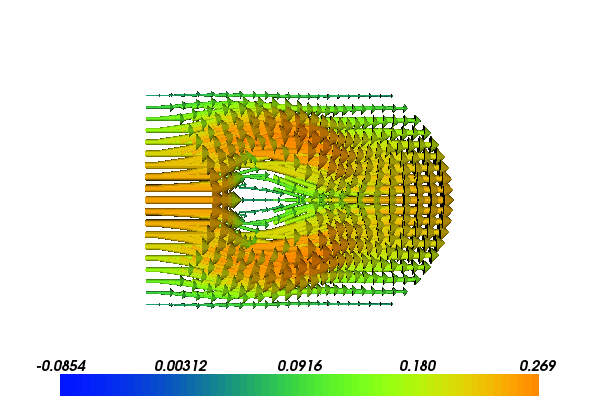
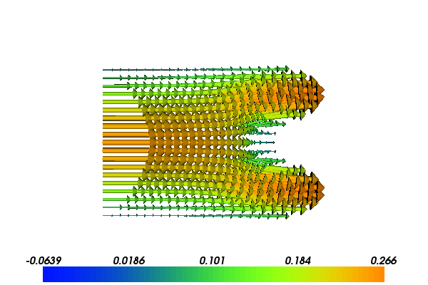
Figure 4: Velocity problem around a porous media with near optimal values: \( K_0=564, x_0 = 0.92, c=0.10 \).
For this particular application we assume that the Reynolds number is low such that the flow can be modeled by the Stokes problem. Furthermore, the additional resistance caused by the porous medium is modeled by a positive lower order term \( K u \) resulting in the Brinkman model. The equations then reads
$$ \begin{align} -\Delta u + K u - \nabla p &= 0,\quad \mbox{ in }\Omega \\ \nabla \cdot u &= 0,\quad \mbox{ in } \Omega \\ u &= (0,0),\quad \mbox{ on } y=0,1 \\ u &= (y(1-y),0),\quad \mbox{ on } x=0 \\ \frac{\partial u}{\partial n} + p n &= 0,\quad \mbox{ on } x=1 \end{align} $$ with
$$ K = K_0 \mbox{ if } |x - x_0 | \leq c,\ | y - 0.5 | \leq c, $$ while \( K=0 \) outside this rectangular region.
When \( K=0 \) we have viscous Stokes flow while inside the porous medium, \( K=K_0 \), and the \( K u \) term in the equation dominates over the viscous term \( \Delta u \).
The goal functional that we seek to minimize is $$ \begin{align} J(K_0, x_0, c) = u_x|_{(x=1,y=0.5)} + \int_\Omega (\nabla p)^2 \, dx \end{align} $$ Here, \( u \) and \( p \) are functions of \( K_0 \), \( x_0 \), and \( c \), and \( u_x \) is the \( x \) component of \( u \).
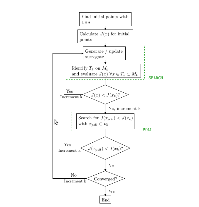
The MATLAB/Octave code for the surrogate management and Kriging is based on Dace, but has been extended by Alison Marsden et. al. cite{Marsden_et_al_2004, Marsden_et_al_2008, Marsden_et_al_2012} to implement surrogate management. This algorithm consists of four main steps 1) search, 2) poll, 3) refine and 4) run simulations, with a flow chart appearing in Figure 5. The two first steps find new sample points \( K_0 \), \( x_0 \), and \( c \), while refine increases the resolution in the parameter space, and finally the fourth step runs simulations with the new sample points.
Figure 5: The flow chart of the surrogate management method.
The main algorithm is implemented in Python (file
opimize_flow_by_SMF.py) and listed below. It
calls three key Python functions: search, poll, and refine,
which make calls to the MATLAB/Octave package.
# main loop
while nit <= max_nit and refine_ok and not converged:
   # search step
   if cost_improve:
       Ai_new = search(Aall, Jall, curr_bestA, theta,
                       upb, lob, N, amin, amax, spc, delta)
       prev_it = "search"
       Ai_new = coarsen(Ai_new)
   else:
       # poll step
       if prev_it == "search":
	   Ai_new = poll(Aall, Jall, curr_bestA, N,
                         delta, spc, amin, amax)
	   prev_it = "poll"
       # refine if previous poll did not lead to cost improvement
       if prev_it == "poll":
	   refine_ok, delta, spc = refine(delta, deltamin, spc)
           if refine_ok:
	       Ai_new = search(Aall, Jall, curr_bestA, theta,
                               upb, lob, N, amin, amax, spc, delta)
	       prev_it = "search"
           else:
               Ai_new = None
   nit += 1

   # run simulations on the new parameters
   if not Ai_new == None:
       Ai_new, J_new = run_simulations(Ai_new)

       # stack the new runs to the previous
       Jall = numpy.hstack((Jall, J_new))
       Aall = numpy.vstack((Aall, Ai_new))

       # monitor convergence (write to files)
       monitor(Aall, Jall, nit, curr_bestA, curr_bestJ,
               delta, prev_it, improve, spc)

       # check convergence
       cost_improve, curr_bestA, curr_bestJ = check(
           Ai_new, J_new, nit, curr_bestJ, curr_bestA)
   else:
       cost_improve = 0
The search and poll steps are both implemented in Python but are mainly wrappers around MATLAB/Octave functions. The search step is implemented as follows:
def search(Aall, Jall, curr_bestA, theta, upb,
           lob, N, amin, amax, spc, delta):
    """Search step."""
     # make sure that all points are unique
    (Am, Jm) = pytave.feval(2, "dsmerge", Aall, Jall)

    next_ptsall = []
    next_pts = None
    max_no_searches = 100
    no_searches = 0
    while next_pts == None and no_searches < max_no_searches:
	next_ptsall, min_est, max_mse_pt = pytave.feval(
            3, "krig_min_find_MADS_oct",
            Am, Jm, curr_bestA, theta, upb, lob,
            N, amin, amax, spc, delta)
	next_pts = check_for_new_points(next_ptsall, Aall)
	no_searches += 1
    return next_pts
Here, dsmerge and krig_min_find_MADS_oct are functions
available in the MATLAB/Octave
files dsmerge.m and krig_min_find_MADS_oct.m. We need to notify
Octave about the directory (SMF) where these files can be found:
pytave.feval(0, "addpath", "SMF")
The FEniCS solver first
defines the inflow condition (class EssentialBC), the K
coefficient in the PDEs, and the Dirichlet boundary:
class EssentialBC(Expression):
    def eval(self, v, x):
        if x[0] < DOLFIN_EPS:
            y = x[1]
            v[0] = y*(1-y);  v[1] = 0
        else:
            v[0] = 0; v[1] = 0

    def value_shape(self):
        return (2,)

class K(Expression):
    def __init__(self, K0, x0, c):
        self.K0, self.x0, self.c = K0, x0, c

    def eval(self, v, x):
        x0, K0, c = self.x0, self.K0, self.c
        if abs(x[0] - x0) <= c and abs(x[1] - 0.5) <= c:
            v[0] = K0
        else:
            v[0] = 1

def dirichlet_boundary(x):
    return bool(x[0] < DOLFIN_EPS or x[1] < DOLFIN_EPS or \
                x[1] > 1.0 - DOLFIN_EPS)
The core of the solver is the following class:
class FlowProblem2Optimize:
    def __init__(self, K0, x0, c, plot):
        self.K0, self.x0, self.c, self.plot = K0, x0, c, plot

    def run(self):
        K0, x0, c = self.K0, self.x0, self.c

        mesh = UnitSquareMesh(20, 20)
        V = VectorFunctionSpace(mesh, "Lagrange", 2)
        Q = FunctionSpace(mesh, "Lagrange", 1)
        W = MixedFunctionSpace([V,Q])
        u, p = TrialFunctions(W)
        v, q = TestFunctions(W)
        k = K(K0, x0, c)

        u_inflow = EssentialBC()
        bc = DirichletBC(W.sub(0), u_inflow, dirichlet_boundary)
        f = Constant(0)

        a = inner(grad(u), grad(v))*dx + k*inner(u, v)*dx + \
            div(u)*q*dx + div(v)*p*dx
        L = f*q*dx

        w = Function(W)
        solve(a == L, w, bc)

        u, p = w.split()
        u1, u2 = split(u)

        goal1 = assemble(inner(grad(p), grad(p))*dx)
        goal2 = u(1.0, 0.5)[0]*1000
        goal = goal1 + goal2

        if self.plot:
            plot(u)

        key_variables = dict(K0=K0, x0=x0, c=c, goal1=goal1,
                             goal2=goal2, goal=goal)
        print key_variables
        return goal1, goal2
It now remains to do the coupling of the optimization algorithm that makes use of MATLAB/Octave files and the FEniCS flow solver. The following function performs the task:
def run_simulations(Ai):
    """Run a sequence of simulations with input parameters Ai."""
    import flow_problem
    plot = True
    if len(Ai.shape) == 1: # only one set of parameters
        J = numpy.zeros(1)
	K0, x0, c = Ai
	p = flow_problem.FlowProblem2Optimize(K0, x0, c, plot)
	goal1, goal2 = p.run()
	J[0] =  goal1 + goal2
    else: # several sets of parameters
        J = numpy.zeros(len(Ai))
        i = 0
	for a in Ai:
	    K0, x0, c = a
	    p = flow_problem.FlowProblem2Optimize(K0, x0, c, plot)
	    goal1, goal2 = p.run()
	    J[i] = goal1 + goal2
	    i = i+1
    return Ai, J
Obviously, Pytave depends on Octave, which can be somewhat challenging to install. Prebuilt binaries are available for Linux (Debian/Ubuntu, Fedora, Gentoo, SuSE, and FreeBSD), Mac OS X (via MacPorts or Homebrew), and Windows (requires Cygwin). On Debian-based systems (including Ubuntu) you are recommended to run these commands
# Install Octave
sudo apt-get update
sudo apt-get install libtool automake libboost-python-dev libopenmpi-dev
sudo apt-get install octave  octave3.2-headers

# Install Pytave
bzr branch lp:pytave
cd pytave
bzr revert -r 51
autoreconf --install
./configure
sudo python setup.py install
Pytave has not yet been officially released, but it is quite stable
and has a rather complete interface to Octave. Unfortunately, the
latest changeset has a bug and that is why we need to revert
to a previous revision (bzr revert -r 51).
There are at least two Python modules that interface MATLAB: pymat2 and pymatlab, but the authors do not have MATLAB installed and were unable to test these packages.
Although FEniCS can easily and flexibly be extended by Python code, the need for speed in scientific computing occasionally makes a demand to implement new finite element functionality in C++. The present example shows how one can extend DOLFIN's finite element functionality through a new piece of C++ code and call this functionality from a Python FEniCS solver.
FEniCS finite element functions can be evaluated at an arbitrary
point in the mesh. In a parallel computing setting, however,
the evaluation point must be in the part of the mesh that belongs
to the current process and the searching for the element containing
the point is not optimally efficient. Therefore, one may want to
have a utility for fast evaluation of finite element functions
at prescribed points on parallel computers.
We can write a class Probe for this purpose. The constructor takes a spatial
point x and precomputes which element that
contains the point and other data useful for later
fast evaluation of functions at x.
A member function eval(u) takes any Function object u and
stores its value(s) at the point x. With get_values(i) we
can retrieve all values component i of the function computed in
previous calls to eval.
For a scalar function there is only one component (i=0), but
the class supports vector and tensor functions too.
The name Probe reflects the use of such a class: we insert a
probe, as in a physical experiment, and measure the response
at that point through time. In FEniCS simulators it means that we
want to record the evolution in time of some field at a given spatial
point. For long time series there can be a lot of evaluations of
the field at this point, and class Probe will be much more
efficient than the standard FEniCS point evaluation of fields (which
performs a lot of searching to find the element containing the point).
Class Probe is a fairly short C++ code that makes use of various
DOLFIN C++ classes and programming conventions. The header file
reads
#include <dolfin/function/FunctionSpace.h>
#include <dolfin/function/Function.h>

namespace dolfin
{
  class Probe
  {
  public:
    Probe(const Array<double>& point, const FunctionSpace& V);
    void eval(const Function& u);
    std::vector<double> get_values(std::size_t component);

    std::size_t num_components() {return value_size_loc;};
    std::size_t number_of_eval_calls() {return _probes[0].size();};
    std::vector<double> get_point();
    void erase(std::size_t i);
    void clear();

  private:
    std::vector<std::vector<double> > basis_matrix;
    std::vector<double> coefficients;
    double _x[3];
    boost::shared_ptr<const FiniteElement> _element;
    Cell* dolfin_cell;
    UFCCell* ufc_cell;
    std::size_t value_size_loc;
    std::vector<std::vector<double> > _probes;
  };
}
The most important functionality for users
lies in the constructor and the eval and get_values functions, while the
rest of the class contains short convenience functions and data
structures for help with fast function evaluations.
Note that eval does not return any value, it just records the
value.
The reader may consult the corresponding Probe.cpp file for all implementation details. Obviously, this type of code requires familiarity with the DOLFIN classes, but looking at the DOLFIN code itself is a good starting point for learning about those classes, the associated implementation conventions, and other programming tools that the DOLFIN library makes use of.
The next, and often more technically challenging, step is to compile
the C++ code, link it to DOLFIN, and make it callable from a FEniCS
solver in Python. Fortunately, this is not so difficult if we use the
FEniCS Just-in-time (JIT) compiler Instant, which is already the
compiler that DOLFIN applies when compiling variational forms. Instant
employs SWIG in its JIT compiling, and some knowledge of SWIG is
therefore required to understand how Instant works. However, hardly
any SWIG knowledge is needed if we use the convenience function
compile_extension_module found in the Python package dolfin
package. This function is a high-level interface to Instant
functionality.
Basically, the compile_extension_module function
requires a declaration of our C++ code to be interfaced, a list
of .cpp source code files, and some information on where files
are found. Compilation and linking are then taken care of automatically.
The C++ code to be interfaced in this example
is contained in the Probe.h header file.
The call to the compile_extension_module function is then
from dolfin import *
import numpy
import os

header_file = open("Probe/Probe.h", "r")
code = header_file.read()
header_file.close()
probe_module = compile_extension_module(
    code=code, source_directory="Probe", sources=["Probe.cpp"],
    include_dirs=[".", os.path.abspath("Probe")])
We can now import probe_module in the forthcoming code and use it
for fast evaluations at some point x:
mesh = UnitCubeMesh(10, 10, 10)
V = FunctionSpace(mesh, 'CG', 1)

x = numpy.array((0.5, 0.5, 0.5))
probe = probe_module.Probe(x, V)

u0 = interpolate(Expression('x[0]'), V)
# Fast evaluation of U0 at x:
probe.eval(u0)
print "The number of probes is ", probe.number_of_eval_calls()
print "The value at ", x, " is ", probe.get_values(0)
To summarize, with compile_extension_module the compilation and
linking of C++ and DOLFIN code to make accessible in Python is a matter
of one function call.
We shall now go into details how the steps above would be done by
using basic Instant only, as this explains how to use Instant for
interfacing C++ code in general. Instant provides the build_module
function for building a Python module out of the C++ code:
compiled_module = instant.build_module(
    code=code,
    source_directory=source_dir,
    additional_declarations=additional_decl,
    system_headers=system_headers,
    include_dirs=include_dirs,
    swigargs=swigargs,
    sources=sources,
    cmake_packages=cmake_packages)
Here,
code is the C++ code that is to be wrapped,source_directory is the directory where the C++ .cpp files are found,additional_declarations are additional declaration needed to
make SWIG behave properly,system_headers is a list of the additional header files needed
for compilation,include_dirs is a list of
additional include directories required for compilation,swigargs is the arguments that shall be passed to SWIG on the
command line,sources is
a list of C++ files that shall be compiled into the Pyhton module, andcmake_packages is a list of packages that the CMake compilation
depend on.
system_headers = ['numpy/arrayobject.h',
                  'dolfin/function/Function.h',
                  'dolfin/function/FunctionSpace.h']
swigargs = ['-c++', '-fcompact', '-O', '-I.', '-small']
cmake_packages = ['DOLFIN']
sources = ["Probe.cpp"]
source_dir = "Probe"
The Probe class employs several DOLFIN classes. Hence, for this class
to work properly it is crucial that the JIT compiler and SWIG are told
how to relate to the DOLFIN classes. Instant provides the hook
additional_declarations for providing additional declarations to
SWIG. Such declarations require knowledge of how to write
SWIG interface files. In the current example, the additional
declarations look like the following string:
additional_decl = """
%init%{
import_array();
%}

// Include global SWIG interface files:
// Typemaps, shared_ptr declarations, exceptions, version
%include <boost_shared_ptr.i>

// Global typemaps and forward declarations
%include "dolfin/swig/typemaps/includes.i"
%include "dolfin/swig/forwarddeclarations.i"

// Global exceptions
%include <exception.i>

// Local shared_ptr declarations
%shared_ptr(dolfin::Function)
%shared_ptr(dolfin::FunctionSpace)

// %import types from submodule function of SWIG module function
%import(module="dolfin.cpp.function") "dolfin/function/Function.h"
%import(module="dolfin.cpp.function") "dolfin/function/FunctionSpace.h"

%feature("autodoc", "1");
"""
The init part containing import_array is always needed when NumPy
[8] arrays are involved. Thereafter, we include various SWIG interface
files (ending in .i) that we need in DOLFIN-related code. We also
need shared pointers for dolfin::Function and
dolfin::FunctionSpace. In addition we need header files for
Function and FunctionSpace classes in DOLFIN. Note that the
import and include statements in SWIG may seem similar, but that
whereas include makes SWIG generate wrappers for the code included,
the import directive simply provides SWIG with the necessary type
information.
We refer to the complete file instant_test_probe.py for how all of the information about is put together and executed in order to build the extension module using plain Instant functionality.
In this final example we will consider a solver for a reaction-diffusion equation described by a parabolic PDE coupled to a set of ODEs. The equation can be written as
$$ \begin{align*} u_t &= \Delta u + f(u, s), & \forall x \in\Omega,\ t>0, \\ s_t &= g(u, s), & \forall x \in \Omega,\ t>0. \end{align*} $$ Here, \( u \) is a scalar function, subscript \( t \) means differentiation with respect to time, \( s \) is a scalar field (governed pointwise by an ODE), and \( \Delta u \) is a Laplace term. The problem is usually solved using a first order operator splitting scheme, where we at a time level first solve the PDE with \( f \) evaluated at the previous time level, and thereafter we update the ODEs using the most recent value of \( u \). More precisely,
$$ \begin{align*} u^n &= u^{n-1} + \Delta t (\Delta u^n + f(u^{n-1}, s^{n-1})), \\ s^n &= s^{n-1} + \Delta t g(u^n, s^{n-1}) , \end{align*} $$ The superscript \( n \) denotes the time level, and \( \Delta t \) is the time step.
The solver for the parabolic problem is implemented in FEniCS, while
the ODE solver is implemented in a homemade C++ code. We will glue
these two different solvers together using Python. The C++ code consists
basically of the class ODEFieldSolver declared in a file
ODEFieldSolver.h:
class ODEFieldSolver {
  int n;                // no of points (or regions)
  double* s;            // discrete values of unknown s)
  double* s_1;          // s at the previous time level
  double* u;            // discrete values of external field u
  double dt;            // time step size

  public:
  ODEFieldSolver();
 ~ODEFieldSolver();
  void redim(int n);    // allocate data structures
  int size();           // return the no of points/regions
  virtual double g(double s, double u);
  void set_dt(double dt);
  void set_IC(int n, double* in_array);
  void set_u (int n, double* in_array);
  void set_IC(double const_value);
  void set_u (double const_value);
  void advance_one_timestep();
};
The set_IC functions set the initial condition of the ODE system, and
set_u provides the \( u \) field (the "environment") to the ODE system.
Note that there are two versions of set_IC and set_u: one for
a constant value one for spatial variations. We refer to
the ODEFieldSolver.cpp
file for implementational details.
The mathematics behind the shown class is to have \( n \) regional or pointwise values of \( u \) and \( s \), and then solve \( s_t = g(s,u) \) in each region or at each point. In the present case we will solve for \( s \) at the nodes in the finite element mesh used to compute \( u \). The \( s \) and \( u \) functions are in the C++ code represented by plain C arrays holding nodal values. The usage of the C++ code typically goes like this:
ODEFieldSolver solver = ODEFieldSolver();
solver.redim(n);               // allocate data
solver.set_dt(dt);             // set time step
solver.set_IC(n, s0);          // set initial conditions
t = 0
while (t <= T) {
    solver.set_u(n, u);        // give access to PDE solution
    solver.advance_one_timestep();
    // plot solver.s
}
A subclass must be written to specify the desired g function.
We need to wrap the C++ class in Python such that
the FEniCS Python solver can call the C++ code.
We would then need to transfer the computed
\( s \) back to Python. To this end, we add a member function get_s
to the class so that we can fill some array on the user's side with
the most recently computed s values:
class ODEFieldSolver {
  ...
  void get_s  (int& n, double* out_array);
};
The easiest way to interface Fortran, C, and C++ code is to use F2PY.
Although F2PY was made for interfacing Fortran and most of the documentation
is written with Fortran codes in mind, it is convenient to interface
C and C++ too. Or more precisely, F2PY can interface a pure C API, not
C++ classes. The idea is then to construct a set of C functions on top
of the C++ classes for accessing high-level operations using the those classes.
The example involving class ODEFieldSolver will illustrate the elements
in this technique.
The first step is to decide on the C API. The exposed functions in Python must do essentially the same as the main program. A possible set of functions is
set_ic_and_dt(int n, double* s0, double dt) for initializing
the class object and setting the initial conditions
and the time step. Also a variant set_const_ic_and_dt for
constant initial condition s0 is handy.set_u(int n, double* u) for assigning the u function to the class.advance_one_timestep() for computing the solution at a time step.get_s(int n, double* s) for getting access to the computed array s
in the ODEFieldSolver class.ODEFieldSolver object and interact with this object as appropriate.
The complete code of the C API then becomes
#include "ODEFieldSolver.h"

ODEFieldSolver solver = ODEFieldSolver();

extern "C" {

void set_ic_and_dt(int n, double* s0, double dt)
{
  solver.redim(n);
  solver.set_dt(dt);
  solver.set_IC(n, s0);
}

void set_const_ic_and_dt(int n, double s0, double dt)
{
  solver.redim(n);
  solver.set_dt(dt);
  solver.set_const_IC(s0);
}

void set_u(int n, double* u)
{
  solver.set_u(n, u);
}

void advance_one_timestep()
{
  solver.advance_one_timestep();
}

void get_s(int n, double* s)
{
  solver.get_s(n, s);
}

}
The nice thing about F2PY is that it can automatically make a Python interface to this C code, where NumPy arrays can be passed to the functions taking plain C arrays as arguments. For this to work, F2PY needs a specification of all the C functions in terms of Fortran 90 module syntax. However, F2PY can generate this module for us if we specify the function signatures in plain Fortran 77. This is done as follows:
      subroutine set_ic_and_dt(n, s0, dt)
Cf2py intent(c) set_ic_and_dt
      integer n
      real*8 s0(0:n-1), dt
Cf2py intent(c) n, s0, dt
      return
      end

      subroutine set_const_ic_and_dt(n, s0, dt)
Cf2py intent(c) set_const_ic_and_dt
      integer n
      real*8 s0, dt
Cf2py intent(c) n, s0, dt
      return
      end

      subroutine set_u(n, u)
Cf2py intent(c) set_u
      integer n
      real*8 u(0:n-1)
Cf2py intent(c) n, u
      return
      end

      subroutine advance_one_timestep()
Cf2py intent(c) advance_one_timestep
      return
      end

      subroutine get_s(n, s)
Cf2py intent(c) get_s
      integer n
Cf2py intent(c) n
      real*8 s(0:n-1)
Cf2py intent(c, in, out) s
      return
      end
For each C function we
CF2PY) that tells that the
function is in C: intent(c),intent(c) (Fortran treats
all arguments as pointers, so the specification of C variables is
strictly needed only for non-pointers),s in get_s as intent(c,in,out),
meaning that we in Python can call this function as s = get_s(s).
The s argument is needed for the function to avoid
reallocating the returned array every time the function is call. Instead
we reuse the storage provied in the s array.
If the Fortran 77 signatures are in a file signatures_capi2cpp.f we
can get F2PY to generate a Fortran 90 module in a file ODEFieldSolvercpp.pyf
by the command
Terminal> F2PY -m ODEFieldSolvercpp -h ODEFieldSolvercpp.pyf \
          --overwrite-signature signatures_capi2cpp.f
The -m option specifies the name of the extension module that contains
the Python interfaces to the C API.
The module typically looks like
!    -*- f90 -*-
! Note: the context of this file is case sensitive.

python module ODEFieldSolvercpp ! in
    interface  ! in :ODEFieldSolvercpp
        subroutine set_ic_and_dt(n,s0,dt)
            intent(c) set_ic_and_dt
            integer, optional,intent(c),check(len(s0)>=n),depend(s0) :: n=len(s0)
            real*8 dimension(n),intent(c) :: s0
            real*8 intent(c) :: dt
        end subroutine set_ic_and_dt
        subroutine set_const_ic_and_dt(n,s0,dt)
            intent(c) set_const_ic_and_dt
            integer intent(c) :: n
            real*8 intent(c) :: s0
            real*8 intent(c) :: dt
        end subroutine set_const_ic_and_dt
        subroutine set_u(n,u)
            intent(c) set_u
            integer, optional,intent(c),check(len(u)>=n),depend(u) :: n=len(u)
            real*8 dimension(n),intent(c) :: u
        end subroutine set_u
        subroutine advance_one_timestep ! in :ODEFieldSolvercpp:signatures_capi2cpp.f
            intent(c) advance_one_timestep
        end subroutine advance_one_timestep
        subroutine get_s(n,s)
            intent(c) get_s
            integer, optional,intent(c),check(len(s)>=n),depend(s) :: n=len(s)
            real*8 dimension(n),intent(c,in,out) :: s
        end subroutine get_s
    end interface
end python module ODEFieldSolvercpp

! This file was auto-generated with f2py (version:2).
! See http://cens.ioc.ee/projects/f2pye/
Those who are familiar with Fortran 90 modules can write such code by hand instead of first writing Fortran 77 headers and letting F2PY generate the module.
With the aid of the Fortran 90 specification of the C functions, F2PY can compile and link the extension module by a command like
Terminal> F2PY -c --fcompiler=gfortran -I.. --build-dir tmp1 \
         -DF2PY_REPORT_ON_ARRAY_COPY=1 \
          ODEFieldSolvercpp.pyf ../ODEFieldSolver.cpp capi2cpp.cpp
The -DF2PY_REPORT_ON_ARRAY_COPY=1 option is handy for letting F2PY
notify us if arrays are copied when transferred from Python to C,
as we want to avoid time-consuming copies. The C++ class is assumed
to be in the parent directory (note -I.. and the ../ prefix
in the filename). All the files generated
and built by F2PY will reside in the tmp1 directory for later
inspection if run into build problems.
The result of the above compile command is a C/C++ extension module
in the file ODEFieldSolvercpp.so. The module can be loaded
into Python and examined for content:
>>> import ODEFieldSolvercpp
>>> dir(ODEFieldSolvercpp)
['__doc__', '__file__', '__name__', '__package__', '__version__',
 'advance_one_timestep', 'get_s', 'set_const_ic_and_dt',
 'set_ic_and_dt', 'set_u']
>>> print ODEFieldSolvercpp.__doc__
This module 'ODEFieldSolvercpp' is auto-generated with F2PY (version:2).
Functions:
  set_ic_and_dt(s0,dt,n=len(s0))
  set_const_ic_and_dt(n,s0,dt)
  set_u(u,n=len(u))
  advance_one_timestep()
  s = get_s(s,n=len(s))
A word of caution is required for newcomers to F2PY: it is extremely
important to study the doc strings of the various functions before
trying to call them from Python. The reason is that F2PY drops
unnecessary arguments, such as array lengths (since these are
contained in NumPy array objects), and all output arguments are
returned and removed from the subroutine's argument list.
The function arguments and return values are therefore different
in Python and C!
For example, the set_ic_and_dt function only needs s0 transferred
from Python since n can be deduced from the F2PY-generated
interface. The signature of this function, as seen from Python,
is then
>>> print ODEFieldSolvercpp.set_ic_and_dt.__doc__
set_ic_and_dt - Function signature:
  set_ic_and_dt(s0,dt,[n])
Required arguments:
  s0 : input rank-1 array('d') with bounds (n)
  dt : input float
Optional arguments:
  n := len(s0) input int
Furthermore, the get_s function has specified its s
argument as input and output (intent(c,in,out)) and the
doc string shows the correct call syntax:
>>> print ODEFieldSolvercpp.get_s.__doc__
get_s - Function signature:
  s = get_s(s,[n])
Required arguments:
  s : input rank-1 array('d') with bounds (n)
Optional arguments:
  n := len(s) input int
Return objects:
  s : rank-1 array('d') with bounds (n)
The Python code for calling the C++ functions in the ODEFieldSolvercpp
module can take the following form:
import ODEFieldSolvercpp as solver
import numpy

s0 = numpy.array([0, 1, 4], float)  # ensure float elements!
u = numpy.array([0, 1, 1], float)
n = s0.size
s = numpy.zeros(n)

solver.set_ic_and_dt(s0, dt=0.1)
for n in range(1, 8):
    solver.set_u(u)
    solver.advance_one_timestep()
    s = solver.get_s(s)
    print n, s
It may be illustrative to also see a pure C code that implements the same type of actions as the C++ class. The class variables are here global variables in a library and all the class functions are stand-alone C functions working with these global variables. A bit more sophisticated implementation would collect the global variables in a global struct instead, so that the functions work with the struct. The advantage of a pure C code is that F2PY can interface all parts of this code directly without any need to make a C API to C++ code. (Having said that, we should add that making a C API to C++ codes is often a good exercise as it tends to emphasize faster computing with arrays rather than with special (potentially small) C++ objects. Python interfacing of C++ this way may lead to sound redesign of the C++ code.)
The pure C implementation goes as follows:
#include <stdlib.h>
#include <stdio.h>

/* global variables */
double* s;
double* s_1;
double* u;
double dt;
int n;

void redim(int n_)
{
  n = n_;
  s =   malloc(sizeof(double)*n);
  s_1 = malloc(sizeof(double)*n);
  u =   malloc(sizeof(double)*n);
}

void deallocate()
{
  free(s); free(s_1); free(u);
}

/* Note: do not mix upper and lower case letters as in set_IC_...
   This leads to undefined symbols when f2py compiles the code.
*/

void set_ic_and_dt(int n_, double* s0, double dt_)
{
  int i;
  redim(n_);
  dt = dt_;
  for (i=0; i<n; i++) {
    s_1[i] = s0[i];
  }
}

void set_const_ic_and_dt(int n_, double s0, double dt_)
{
  int i;
  redim(n_);
  dt = dt;
  for (i=0; i<n; i++) {
    s_1[i] = s0;
  }
}

void set_u(int n_, double* u_)
{
  int i;
  for (i=0; i<n; i++) {
    u[i] = u_[i];
  }
}

double g(double s_, double u_) {
  /* return s_*u_*(1 - s_); */
  return s_;
}

void advance_one_timestep()
{
  /* Use the Forward Euler time integration for simplicity */
  int i;
  for (i=0; i<n; i++) {
    s[i] = s_1[i] + dt*g(s_1[i], u[i]);
    /* For debugging: */
    /* printf("i=%d, s_1=%g, dt=%g, g=%g, s=%g\n",
       i, s_1[i], dt, g(s_1[i], u[i]), s[i]); */
  }
  /* Update for next time step */
  for (i=0; i<n; i++) { s_1[i] = s[i]; }

}

void get_s(int n_, double* s_)
{
  int i;
  for (i=0; i<n; i++) {
    s_[i] = s[i];
  }
}
By writing the corresponding Fortran 77 signatures, F2PY can generate a Fortran 90 module specification of the extension module, and this code can be compiled as explained above. We refer to the files in the f2py-c directory for details.
Next, we employ the tool SWIG to wrap the C++ class directly and make it available as a Python class. SWIG is also used in DOLFIN and Instant, as demonstrated in the section How to interface a C++/DOLFIN code from Python. Useful references on SWIG in a FEniCS context are [2] [9] [10] [11].
To use SWIG, you must first write an interface file (ending in .i)
that tells SWIG about the parts of the C++ code you want to access
from Python. The next step is to run SWIG to generate (a lot of) wrapper
code in C. The final step is to compile the wrapper code and your C++ code
and link with required libraries.
A first attempt to write an interface for our ODEFieldSolver class
consists in listing just the class declaration:
%module ODEFieldSolver
%{
#include <arrayobject.h>
#include <sstream>
#include "ODEFieldSolver.h"
%}


%init %{
import_array();
%}

class ODEFieldSolver {
  int n;                // no of points (or regions)
  double* s;            // discrete values of unknown s)
  double* s_1;          // s at the previous time level
  double* u;            // discrete values of external field u
  double dt;            // time step size

  public:
  ODEFieldSolver();
 ~ODEFieldSolver();
  void redim(int n);    // allocate data structures
  int size();           // return the no of points/regions
  virtual double g(double s, double u);
  void set_dt(double dt);
  void set_IC(int n, double* in_array);
  void set_u (int n, double* in_array);
  void set_IC(double const_value);
  void set_u (double const_value);
  void advance_one_timestep();

  void get_s  (int& n, double* out_array);
};
All SWIG commands start with %. The %module command defines the
name of the module. Following this command comes a list of header files
needed by the module. The %init command includes code that should be
executed when the module is imported in Python. When using NumPy arrays
in C++ code we always need to call the import_array function to
initialize the NumPy package (removal of this statement will
result in a segmentation fault!). The rest of the code defines the
interface that should be wrapped, that is; the declaration of the
class ODEFieldSolver.
SWIG is meant to automate interfacing of C and C++ code, and there is
mainly only one thing that needs to be addressed manually: the
handling of pointers to arrays. Consider for instance the set_IC
function. Here, in_array is a pointer to the first element of a
double precision array of length n. However, the fact that
in_array is an array is not explicitly stated in C++, and therefore
SWIG simply by default handles the pointer as a plain pointer, and
this is not what we want. SWIG does, however, offer typemaps for
changing this default behavior. With typemaps we can specify that the
pointer in_array is a NumPy array object (PyObject) when it comes
from Python, and we can extract the underlying data pointer
(double*) and communicate it to C.
To enable NumPy arrays to be passed to the functions set_IC and
set_u we provide the following typemap.
%typemap(in) (int n, double* array){
  if (!PyArray_Check($input)) {
    PyErr_SetString(PyExc_TypeError, "Not a NumPy array");
    return NULL; ;
  }
  PyArrayObject* pyarray;
  pyarray = (PyArrayObject*)$input;
  if (!(PyArray_TYPE(pyarray) == NPY_DOUBLE)) {
    PyErr_SetString(PyExc_TypeError, "Not a NumPy array of doubles");
    return NULL; ;
  }
  $1 = int(pyarray->dimensions[0]);
  $2 = (double*)pyarray->data;
}
Typemap code often looks complicated, at least when viewed for the
first time. The logic is straightforward, though, once some basic
knowledge of the C API of Python and NumPy is acquired. The idea
with the typemap is to recognize a set of arguments in C/C++, here
n and in_array, and then execute some C/C++ code to transform
a Python object to the C/C++ arguments.
In the present example we want to map a NumPy array object
to an integer n (the array size) and a plain C array in_array
(the array data). All Python objects, when viewed in C, are of type
PyObject. We can think of PyObject as a superclass for all the different
object types in Python. The special NumPy array object type is
PyArrayObject.
SWIG has some special variables prefixed with $, which in the
present example are $input for the incoming NumPy array object, and
$1 and $2 for the outgoing C/C++ arguments n and in_array.
The first if statement checks that the incoming array is of right
type, and if not, a TypeError exception is raised. The return
NULL statement is essential for this exception to work. The next
step is to cast the PyObject pointer in $input to the correct
array object type, PyArrayObject, because we need this object to
call C functionality in the NumPy object to extract the data and the
array size. For safety reasons, we insert a test that the array data
are of type NPY_DOUBLE so that the array element types in Python and
C match. Then we come to the final and most essential point:
extracting data from the NumPy array object and storing them in n
($1) and in_array ($2):
$1 = int(pyarray->dimensions[0]);
$2 = (double*)pyarray->data;
Because we have overloaded the set_IC function, we also need to provide
SWIG with a typecheck to determine which of the C++ functions to use.
A suitable typecheck is:
%typecheck(SWIG_TYPECHECK_DOUBLE_ARRAY) (int n, double* array) {
$1 = PyArray_Check($input) ? 1 : 0;
}
The function
void get_s(int n, double *array);
should return NumPy arrays when called from Python as
s = odesolver.get_s()
That is, we would like to be able to call this function from Python
without providing and input array, and instead get an output
array. This means that an array must be created before being passed to
C++ and then returned to Python. To accomplish this we hide the
function by calling it _get_s. Then we extend the interface using
the %extend and %pythoncode directives with a Python function
get_s. The Python function get_s allocate an array before passing
it to the hidden _get_s function and thereafter it
returns the array. The code is
/* Wrap ODEFieldSolver::get_s in a Python function */
%rename (_get_s) ODEFieldSolver::get_s;
%extend ODEFieldSolver{
%pythoncode%{
def get_s(self):
import numpy as np
a = np.zeros(self.size())
self._get_s(a)
return a
%}
}
To summarize, the complete
SWIG interface file for wrapping the ODEFieldSolver class is
listed next.
%module ODEFieldSolver
%{
#include <arrayobject.h>
#include <sstream>
#include "ODEFieldSolver.h"
%}
%init %{
import_array();
%}
%typecheck(SWIG_TYPECHECK_DOUBLE_ARRAY) (int n, double* array) {
$1 = PyArray_Check($input) ? 1 : 0;
}
%typemap(in) (int n, double* array){
if (!PyArray_Check($input)) {
PyErr_SetString(PyExc_TypeError, "Not a NumPy array");
return NULL; ;
}
PyArrayObject* pyarray;
pyarray = (PyArrayObject*)$input;
if (!(PyArray_TYPE(pyarray) == NPY_DOUBLE)) {
PyErr_SetString(PyExc_TypeError, "Not a NumPy array of doubles");
return NULL; ;
}
  $1 = int(pyarray->dimensions[0]);
  $2 = (double*)pyarray->data;
}
/* Wrap ODEFieldSolver::get_s in a Python function */
%rename (_get_s) ODEFieldSolver::get_s;

%extend ODEFieldSolver{
 %pythoncode%{
    def get_s(self):
      import numpy as np
      a = np.zeros(self.size())
      self._get_s(a)
      return a
 %}
}
%include std_string.i
%include "ODEFieldSolver.h"
To make SWIG generate the wrapper code, we run
swig -python -c++ -I. -I.. ODEFieldSolver.i
SWIG supports many languages and we therefore specify what languages
we need wrapper code for by the -python and -c++ flags. Further,
-I is used to specify where SWIG should look for interface files
(with extension .i). The C++ class files are located in the parent
directory. SWIG will from this command generate two files
ODEFieldSolver.py and ODEFieldSolver_wrap.cxx. The latter needs to
be compiled and linked with the ODEFieldSolver code to form a shared
library with name _ODEFieldSolver.so. The ODEFieldSolver.py file
is the module to use from Python and this is nothing but a Python
class wrapper to _ODEFieldSolver.so module. Building the shared
library is most conveniently done via a standard setup.py
script. The following setup.py file provides an
appropriate recipe for writing this kind of files:
import os, numpy
from distutils.core import setup, Extension
name = 'ODEFieldSolver'
swig_cmd ='swig -python   -c++  -I.. -I.  %s.i' % name
os.system(swig_cmd)
sources = ['../%s.cpp' % name, '%s_wrap.cxx' % name]
setup(name=name,
      ext_modules= [
          Extension('_' + name,
                    sources,
                    include_dirs=['..',
                                  numpy.get_include() + "/numpy"])])
To create and install the extension module
locally in the current working directory (.),
we run
python setup.py install --install-platlib=.
Now we can do import ODEFieldSolver in Python and access the
C++ class as a Python class.
The FEniCS solver for the parabolic PDE can be implemented as a class:
class ParabolicSolver:
  def __init__(self, N, dt):
    """Set up PDE problem for NxN mesh and time step dt."""
    from dolfin import UnitSquareMesh, FunctionSpace, TrialFunction, \
         TestFunction, Function, dx, dot, grad

    mesh = UnitSquareMesh(N,N)
    self.V = V = FunctionSpace(mesh, "Lagrange", 1)

    u = TrialFunction(V)
    v = TestFunction(V)

    a = u*v*dx + dt*dot(grad(u), grad(v))*dx

    self.a = a
    self.dt = dt
    self.mesh = mesh
    self.U = Function(V)

  def advance_one_timestep(self, f, u_1):
    """
    Solve the PDE for one time step.
    f: the source term in the PDE.
    u_1: solution at the previous time step.
    """
    from dolfin import TestFunction, dx, solve

    V, a, dt = self.V, self.a, self.dt  # strip off self prefix
    v = TestFunction(V)
    L = (u_1 + dt*f)*v*dx

    solve(self.a == L, self.U)
    return self.U
The following pseudo code illustrates how to work with this code and the ODE solver:
for i in range(num_time_steps):   # time loop
    <compute f>
    <call ParabolicSolver's advance_one_time_step>
    <compute g>
    <call the ODE solver>
A complete code goes as follows:
import dolfin
import numpy

def F(S, U):
  if isinstance(S, dolfin.Function) and isinstance(U, dolfin.Function):
    from dolfin import *
    f = sin(S)*exp(U)
    return f
  if isinstance(S, numpy.ndarray) and isinstance(U, numpy.ndarray):
    from numpy import *
    f = sin(S)*exp(U)
    return f

class ParabolicSolver:
  def __init__(self, N, dt):
    """Set up PDE problem for NxN mesh and time step dt."""
    from dolfin import UnitSquareMesh, FunctionSpace, TrialFunction, \
         TestFunction, Function, dx, dot, grad

    mesh = UnitSquareMesh(N,N)
    self.V = V = FunctionSpace(mesh, "Lagrange", 1)

    u = TrialFunction(V)
    v = TestFunction(V)

    a = u*v*dx + dt*dot(grad(u), grad(v))*dx

    self.a = a
    self.dt = dt
    self.mesh = mesh
    self.U = Function(V)

  def advance_one_timestep(self, f, u_1):
    """
    Solve the PDE for one time step.
    f: the source term in the PDE.
    u_1: solution at the previous time step.
    """
    from dolfin import TestFunction, dx, solve

    V, a, dt = self.V, self.a, self.dt  # strip off self prefix
    v = TestFunction(V)
    L = (u_1 + dt*f)*v*dx

    solve(self.a == L, self.U)
    return self.U

import dolfin
import numpy

N = 12     # mesh partition
dt = 0.01  # time step
parabolicsolver = ParabolicSolver(N, dt)
U1 = dolfin.Function(parabolicsolver.V)
U0 = dolfin.Function(parabolicsolver.V)
U0.vector()[:] = numpy.random.random(parabolicsolver.V.dim())

Q = dolfin.FunctionSpace(parabolicsolver.mesh, "DG", 0)
S0_ex = dolfin.Expression("x[0]")
S0 = dolfin.interpolate(S0_ex, Q)
S1 = dolfin.Function(Q)

import ODEFieldSolver  # import module wrapping the ODE solver
odesolver = ODEFieldSolver.ODEFieldSolver()
odesolver.redim(S0.vector().size(0))
odesolver.set_IC(S0.vector().array())
plot = True

for i in range(0, 23):  # time loop
  f = F(S0, U0)
  U1 = parabolicsolver.advance_one_timestep(f, U0)

  U1c = dolfin.project(U1, Q)

  odesolver.set_u(U1c.vector().array())
  odesolver.advance_one_timestep()
  S1.vector()[:] = odesolver.get_s()

  U0 = U1
  S0 = S1

  if plot:
    dolfin.plot(U1, title="U")
    dolfin.plot(S1, title="S")
    dolfin.interactive()
Cython can also be used to wrap C/C++ code.
To this end we define the C++ class in a .pyx file:
cimport numpy as cnp
import numpy as np

cdef extern from "ODEFieldSolver.h":

    cppclass ODEFieldSolver_ "ODEFieldSolver":
        ODEFieldSolver()
        void redim(int n)
        int size()
        double g(double s, double u)
        void set_dt(double dt)
        void set_IC(int n, double* array)
        void set_const_IC(double s0)
        void set_u (int n, double* array)
        void set_IC(double val)
        void set_u (double const_value)
        void advance_one_timestep()
        void get_s  (int n, double* array)
Here, we redefine the name to ODEFieldSolver_ such that we may shadow the
underlying class with the following Python class:
cdef class ODEFieldSolver:
    cdef ODEFieldSolver_  *wrapped

    def __init__(self):
        self.wrapped = new ODEFieldSolver_()

    def __dealloc__(self):
        if self.wrapped != NULL:
            del self.wrapped
We have a pointer called wrapped to the underlying SWIG-generated
C interface to the C++ code.
Simple functions like e.g. redim are straightforward to wrap,
    def redim(self, n):
        self.wrapped.redim(n)
For the set_IC function we need to check that the input argument is a contiguous 1-dimensional numpy array
of type double. This is spesified as cnp.ndarray[double, ndim=1, mode='c']. Further, we check that
the length of the input array is the same as self.wrapped.size before we pass the input array to the
underlying C++ object.
    def set_IC(self, cnp.ndarray[double, ndim=1, mode='c'] array):
        if array.shape[0] != self.wrapped.size():
            raise ValueError('incorrect dimension on array')
        self.wrapped.set_IC(array.shape[0], &array[0])
We allow the user to employ the get_s function both with and without an input
argument, refered to as out. If the user does not supply any input,
i.e., if out is None then we create an array of appropriate type and size. Otherwise,
we check that out has the appropriate type and size before the array is passed to
the C++ object's get_s function. At the end, we simply return out.
    def get_s(self,
              cnp.ndarray[double, ndim=1, mode='c'] out=None):
        if out is None:
            out = np.empty(self.wrapped.size(), dtype=np.double)
        elif out.shape[0] != self.wrapped.size():
            raise ValueError('incorrect dimension on out')
        self.wrapped.get_s(out.shape[0], &out[0])
        return out
Finally, the module is built using a setup.py script for mixing Python, Cython, and C++ code:
from distutils.core import setup
from distutils.extension import Extension
from Cython.Distutils import build_ext

setup(
    cmdclass = {'build_ext': build_ext},
    ext_modules = [Extension("ODEFieldSolver",
                             ["ODEFieldSolver.pyx", "../ODEFieldSolver.cpp"],
                             include_dirs=['..'],
                             language='c++')]
)