On Schemes for Exponential Decay

Hans Petter Langtangen [1, 2] (hpl at simula.no)

[1] Center for Biomedical Computing, Simula Research Laboratory [2] Department of Informatics, University of Oslo

Sep 24, 2015

Goal

The primary goal of this demo talk is to demonstrate how to write talks with DocOnce and get them rendered in numerous HTML formats.

Layout.

This version utilizes deck slides with the theme sandstone.firefox.

Notice.

Speaker notes show up by pressing "n".

The talk investigates the accuracy of three finite difference schemes for the ordinary differential equation $ u'=-au $ with the aid of numerical experiments. Numerical artifacts are in particular demonstrated.

Problem setting and methods

We aim to solve the (almost) simplest possible differential equation problem

$$ \begin{align} u'(t) &= -au(t) \tag{1}\\ u(0) &= I \tag{2} \end{align} $$

Here,

$ t\in (0,T] $

$ a $, $ I $, and $ T $ are prescribed parameters

$ u(t) $ is the unknown function

The ODE (1) has the initial condition (2)

The ODE problem is solved by a finite difference scheme

Mesh in time: $ 0= t_0 < t_1 \cdots < t_N=T $

Assume constant $ \Delta t = t_{n}-t_{n-1} $

$ u^n $: numerical approx to the exact solution at $ t_n $

The $ \theta $ rule,

$$ u^{n+1} = \frac{1 - (1-\theta) a\Delta t}{1 + \theta a\Delta t}u^n, \quad n=0,1,\ldots,N-1 $$

contains the Forward Euler ($ \theta=0 $), the Backward Euler ($ \theta=1 $), and the Crank-Nicolson ($ \theta=0.5 $) schemes.

The Forward Euler scheme explained

Implementation

Implementation in a Python function:

def solver(I, a, T, dt, theta):
    """Solve u'=-a*u, u(0)=I, for t in (0,T]; step: dt."""
    dt = float(dt)           # avoid integer division
    N = int(round(T/dt))     # no of time intervals
    T = N*dt                 # adjust T to fit time step dt
    u = zeros(N+1)           # array of u[n] values
    t = linspace(0, T, N+1)  # time mesh

    u[0] = I                 # assign initial condition
    for n in range(0, N):    # n=0,1,...,N-1
        u[n+1] = (1 - (1-theta)*a*dt)/(1 + theta*dt*a)*u[n]
    return u, t

How to use the solver function

A complete main program.

# Set problem parameters
I = 1.2
a = 0.2
T = 8
dt = 0.25
theta = 0.5

from solver import solver, exact_solution
u, t = solver(I, a, T, dt, theta)

import matplotlib.pyplot as plt
plt.plot(t, u, t, exact_solution)
plt.legend(['numerical', 'exact'])
plt.show()

The Crank-Nicolson method shows oscillatory behavior for not sufficiently small time steps, while the solution should be monotone

The artifacts can be explained by some theory

Exact solution of the scheme:

$$ u^n = A^n,\quad A = \frac{1 - (1-\theta) a\Delta t}{1 + \theta a\Delta t}\thinspace .$$

Key results:

Stability: $ |A| < 1 $

No oscillations: $ A>0 $

$ \Delta t < 1/a $ for Forward Euler ($ \theta=0 $)

$ \Delta t < 2/a $ for Crank-Nicolson ($ \theta=1/2 $)

Concluding remarks:

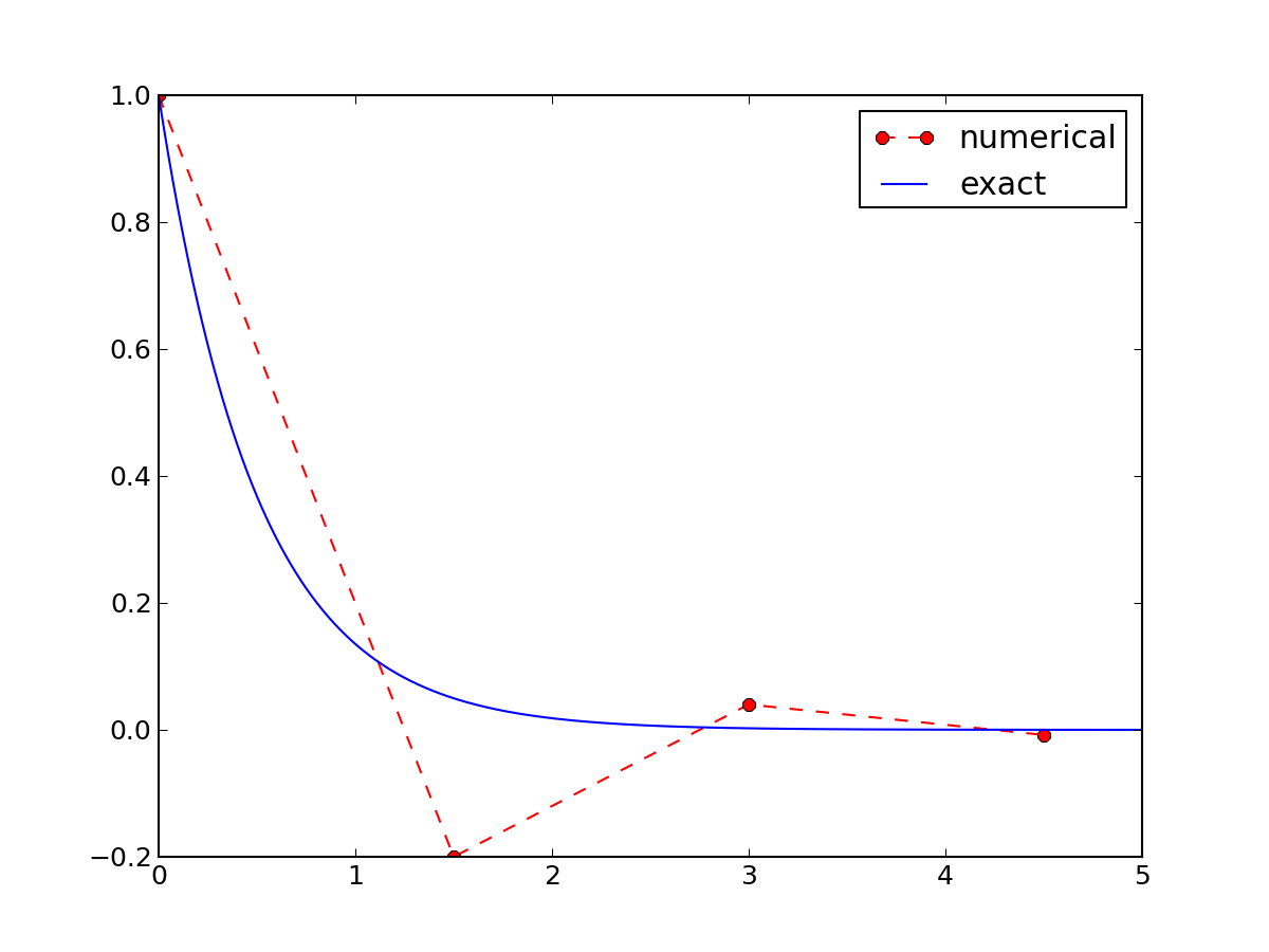
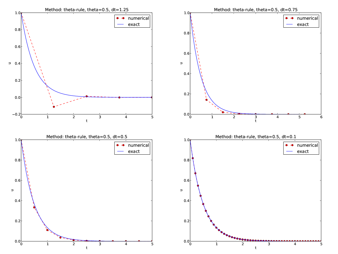
Only the Backward Euler scheme is guaranteed to always give qualitatively correct results.