Modeling the Spreading of Diseases
Nov 20, 2015
We shall model a very complex phenomenon by simple math....
- We consider a perfectly mixed population in a confined area
- No spatial transport, just temporal evolution
- We do not consider individuals, just a grand mix of them
(cf. statistical mechanics vs thermodynamics)
We consider very simple models, but these can be extended to full models that are used world-wide by health authorities. Typical diseases modeled are flu, measles, swine flu, HIV, ...
All these slides and associated programs are available from https://github.com/hplgit/disease-modeling.
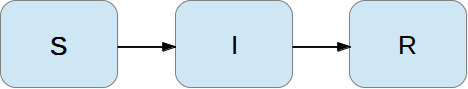
We keep track of 3 categories in the SIR model
- S: susceptibles - who can get the disease
- I: infected - who have developed the disease and infect susceptibles
- R: recovered - who have recovered and become immune
\( S(t) \), \( I(t) \), \( R(t) \): no of people in each category
Find and solve equations for \( S(t) \), \( I(t) \), \( R(t) \)
The traditional modeling approach is very mathematical - our idea is to model, program and experiment
- Numerous books on mathematical biology treat the SIR model
- Quick modeling step (max 2 pages)
- Nonlinear differential equation model
- Cannot solve the equations, so focus is on discussing stability (eigenvalues), qualitative properties, etc.
- Very few extensions of the model to real-life situations
Dynamics in a time interval \( \Delta t \): \( \Delta t\,\beta SI \) people move from S to I
- In a mix of S and I people, there are \( SI \) possible pairs
- A certain fraction \( \Delta t\,\beta \) of \( SI \) meet in a (small) time interval \( \Delta t \), with the result that the infected "successfully" infects the susceptible
- The loss \( \Delta t\,\beta SI \) in the S catogory is a corresponding gain in the I category
It is reasonable that the fraction depends on \( \Delta t \) (twice as many infected in \( 2\Delta t \) as in \( \Delta t \)). \( \beta \) is some unknown parameter we must measure, supposed to not depend on \( \Delta t \), but maybe time \( t \). \( \beta \) lumps a lot of biological and sociological effects into one number.
For practical calculations, we must express the S-I interaction with symbols
Loss in \( S(t) \) from time \( t \) to \( t+\Delta t \):
$$ S(t+\Delta t) = S(t) - \Delta t\,\beta S(t)I(t)$$
Gain in \( I(t) \):
$$ I(t+\Delta t) = I(t) + \Delta t\,\beta S(t)I(t)$$
Modeling the interaction between R and I
- After some days, the infected has recovered and moves to the R category
- A simple model: in a small time \( \Delta t \) (say 1 day), a fraction \( \Delta t\,\nu \) of the infected are removed (\( \nu \) must be measured)
We must subtract this fraction in the balance equation for \( I \):
$$ I(t+\Delta t) = I(t) + \Delta t\,\beta S(t)I(t) -\Delta t\,\nu I(t) $$
The loss \( \Delta t\,\nu I \) is a gain in \( R \):
$$ R(t+\Delta t) = R(t) + \Delta t\,\nu I(t)$$
We have three equations for \( S \), \( I \), and \( R \)
$$
\begin{align}
S(t+\Delta t) &= S(t) - \Delta t\,\beta S(t)I(t)
\tag{1}\\
I(t+\Delta t) &= I(t) + \Delta t\,\beta S(t)I(t) -\Delta t\nu I(t)
\tag{2}\\
R(t+\Delta t) &= R(t) + \Delta t\,\nu I(t)
\tag{3}
\end{align}
$$
Before we can compute with these, we must
- know \( \beta \) and \( \nu \)
- know \( S(0) \) (many), \( I(0) \) (few), \( R(0) \) (0?)
- choose \( \Delta t \)
The computation involves just simple arithmetics
- Set \( \Delta t=6 \) minutes
- Set \( \beta =0.0013 \), \( \nu =0.8333 \)
- Set \( S(0)=50 \), \( I(0)=1 \), \( R(0)=0 \)
$$
\begin{align*}
S(\Delta t) &= S(0) - \Delta t\,\beta S(0)I(0)\approx 49.99\\
I(\Delta t) &= I(0) + \Delta t\,\beta S(0)I(0) -\Delta t\,\nu I(0)\approx 1.002\\
R(\Delta t) &= R(0) + \Delta t\,\nu I(0)\approx 0.0008333
\end{align*}
$$
- In reality, \( S \), \( I \), \( R \) are integers and events are discrete (meet, get sick)
- In the model, we work with real numbers and continuous events
- Reasonable approximation in a not too small population
And we can continue...
$$
\begin{align*}
S(2\Delta t) &= S(\Delta t) - \Delta t\,\beta S(\Delta t)I(\Delta t)\approx 49.87\\
I(2\Delta t) &= I(\Delta t) + \Delta t\,\beta S(\Delta t)I(\Delta t) -\Delta t\,\nu I(\Delta t)\approx 1.011\\
R(2\Delta t) &= R(\Delta t) + \Delta t\,\nu I(\Delta t)\approx 0.00167
\end{align*}
$$
Repeat...
$$
\begin{align*}
S(3\Delta t) &= S(2\Delta t) - \Delta t\,\beta S(2\Delta t)I(2\Delta t)\approx 49.98\\
I(3\Delta t) &= I(2\Delta t) + \Delta t\,\beta S(2\Delta t)I(2\Delta t) -\Delta t\,\nu I(2\Delta t)\approx 1.017\\
R(3\Delta t) &= R(2\Delta t) + \Delta t\,\nu I(2\Delta t)\approx 0.0025
\end{align*}
$$
But this is getting boring! Let's ask a computer to do the work!
First, some handy notation
$$ S^n = S(n\Delta t),\quad I^n = I(n\Delta t),\quad R^n = R(n\Delta t)$$
$$ S^{n+1} = S((n+1)\Delta t),\quad I^{n+1} = I((n+1)\Delta t),\quad R^{n+1} = R((n+1)\Delta t)$$
The equations can now be written more compactly (and computer friendly):
$$
\begin{align}
S^{n+1} &= S^n - \Delta t\,\beta S^nI^n
\tag{4}\\
I^{n+1} &= I^n + \Delta t\,\beta S^nI^n -\Delta t\,\nu I^n
\tag{5}\\
R^{n+1} &= R^n + \Delta t\,\nu I^n
\tag{6}
\end{align}
$$
With variables, arrays, and a loop we can program
Suppose we want to compute until \( t=N\Delta t \), i.e., for \( n=0,1,\ldots,N-1 \). We can store \( S^0, S^1, S^2, \ldots, S^N \) in an array (or list).
Python (Matlab):
t = linspace(0, N*dt, N+1)  # all time points
S = zeros(N+1)
I = zeros(N+1)
R = zeros(N+1)

for n in range(N):
    S[n+1] = S[n] - dt*beta*S[n]*I[n]
    I[n+1] = I[n] + dt*beta*S[n]*I[n] - dt*nu*I[n]
    R[n+1] = R[n] + dt*nu*I[n]
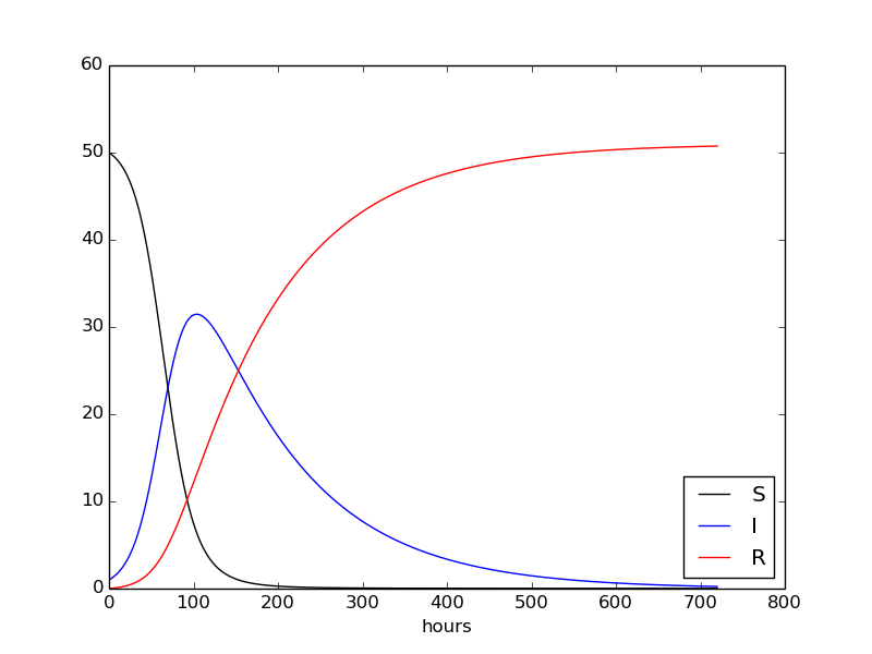
Here is the complete program
beta = 0.0013
nu =0.8333
dt = 0.1             # 6 min (time measured in hours)
D = 30               # simulate for D days
N = int(D*24/dt)     # corresponding no of hours

from numpy import zeros, linspace
t = linspace(0, N*dt, N+1)
S = zeros(N+1)
I = zeros(N+1)
R = zeros(N+1)

for n in range(N):
    S[n+1] = S[n] - dt*beta*S[n]*I[n]
    I[n+1] = I[n] + dt*beta*S[n]*I[n] - dt*nu*I[n]
    R[n+1] = R[n] + dt*nu*I[n]

# Plot the graphs
from matplotlib.pyplot import *
plot(t, S, 'k-', t, I, 'b-', t, R, 'r-')
legend(['S', 'I', 'R'], loc='lower right')
xlabel('hours')
show()
We have predicted a disease!
How much math and programming did we use?
- Plain arithmetics
- The concept of a graph (i.e., discrete function in time)
- Units
- Greek letters
- Variable
- Array
- Loop
- Plotting
Detour: The standard mathematical approach
We had from intuition established
$$
\begin{align*}
S(t+\Delta t) &= S(t) - \Delta t\,\beta S(t)I(t)\\
I(t+\Delta t) &= I(t) + \Delta t\,\beta S(t)I(t) -\Delta t\,\nu I(t)\\
R(t+\Delta t) &= R(t) + \Delta t\,\nu I(t)
\end{align*}
$$
The mathematician will now make differential equations. Divide by \( \Delta t \) and rearrange:
$$
\begin{align*}
\frac{S(t+\Delta t) - S(t)}{\Delta t} &= - \beta S(t)I(t)\\
\frac{I(t+\Delta t) - I(t)}{\Delta t} &= \beta t S(t)I(t) -\nu I(t)\\
\frac{R(t+\Delta t) - R(t)}{\Delta t} &= \nu R(t)
\end{align*}
$$
A derivative arises as \( \Delta t\rightarrow 0 \)
In any calculus book, the derivative of \( S \) at \( t \) is defined as
$$ S'(t) = \lim_{t\rightarrow 0}\frac{S(t+\Delta t) - S(t)}{\Delta t}$$
If we let \( \Delta t\rightarrow 0 \), we get derivatives on the left-hand side:
$$
\begin{align*}
S'(t) &= - \beta S(t)I(t)\\
I'(t) &= \beta t S(t)I(t) -\nu I(t)\\
R'(t) &= \nu R(t)
\end{align*}
$$
This is a 3x3 system of differential equations for the functions \( S(t) \), \( I(t) \), \( R(t) \). For a unique solution, we need \( S(0) \), \( I(0) \), \( R(0) \).
Bad news: we cannot solve these equations!
Replace the derivative with a finite difference, e.g.,
$$ S'(t) \approx \frac{S(t+\Delta t) - S(t)}{\Delta t}$$
which is accurate for small \( \Delta t \).
This brings us back to the first model, which we can solve on a computer!
Parameter estimation is needed for predictive modeling
- Any small \( \Delta t \) will do
- One can reason about \( \nu \) and say that \( 1/\nu \) is the mean recovery time for the disease (e.g., 1 week for a flu)
- \( \beta \) must in some way be measured, but we don't know what it means...
- Can still learn about the dynamics of diseases
- Can find the sensitivity to and influence of \( \beta \)
- Can apply parameter estimation procedures to fit \( \beta \) to data
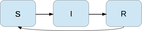
Let us extend the model: no life-long immunity
After some time, people in the R category lose the immunity. In a small time \( \Delta t \) this gives a leakage \( \Delta t\,\gamma R \) to the S category. (\( 1/\gamma \) is the mean time for immunity.)
$$
\begin{align}
S^{n+1} &= S^n - \Delta t\,\beta S^nI^n + {\color{red}\Delta t\,\gamma R^n}
\tag{7}\\
I^{n+1} &= I^n + \Delta t\,\beta S^nI^n -\Delta t\,\nu I^n
\tag{8}\\
R^{n+1} &= R^n + \Delta t\,\nu R^n - {\color{red}\Delta t\,\gamma R^n}
\tag{9}
\end{align}
$$
No complications in the computational model!
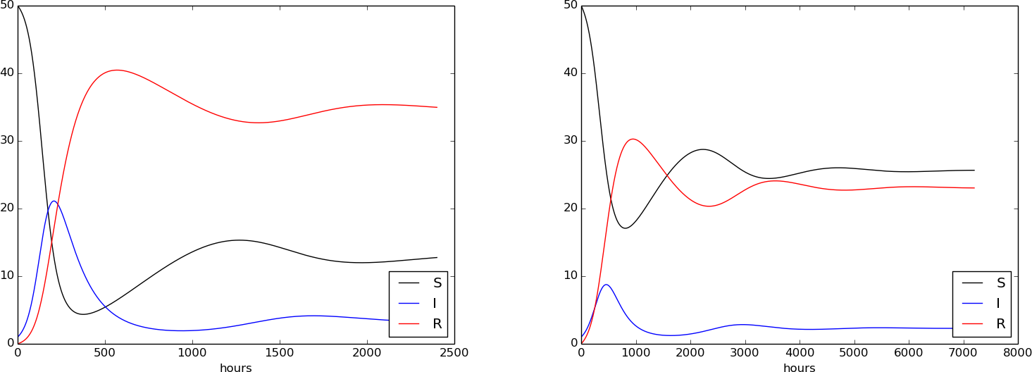
The effect of loss of immunity
\( 1/\gamma = 50 \) days. \( \beta \) reduced by 2 and 4 (left and right, resp.):
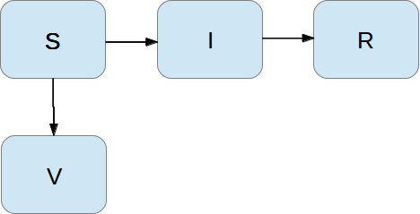
What is the effect of vaccination?
A fraction \( p \) of the S category, per time unit, is vaccinated with success. Then in time \( \Delta t \), \( p\Delta t S \) will move to a vaccinated category, V. This does not affect the I and R categories.
$$
\begin{align}
S^{n+1} &= S^n - \Delta t\,\beta S^nI^n + \Delta t\,\gamma R^n - {\color{red}p\Delta t S^n}
\tag{10}\\
V^{n+1} &= V^n + {\color{red}p\Delta t S^n}
\tag{11}\\
I^{n+1} &= I^n + \Delta t\,\beta S^nI^n -\Delta t\,\nu I^n
\tag{12}\\
R^{n+1} &= R^n + \Delta t\,\nu R^n - \Delta t\,\gamma R^n
\tag{13}
\end{align}
$$
Implementation: Just add array for \( V^n \) and add equation.
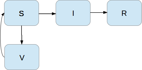
Many possibilities for adjusting the model...
The effect of vaccination decreases over time, so we may move people back to the S category (term proportional to \( \Delta t V \)).
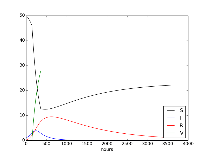
Effect of adding vaccination
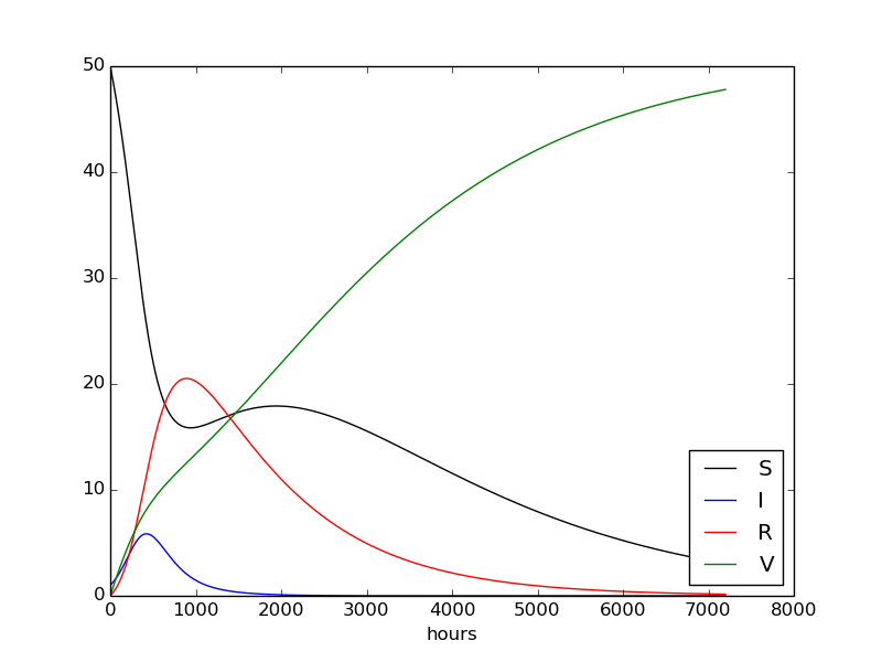
(\( p=0.0005 \))
What is the effect of an intensive vaccination campaign?
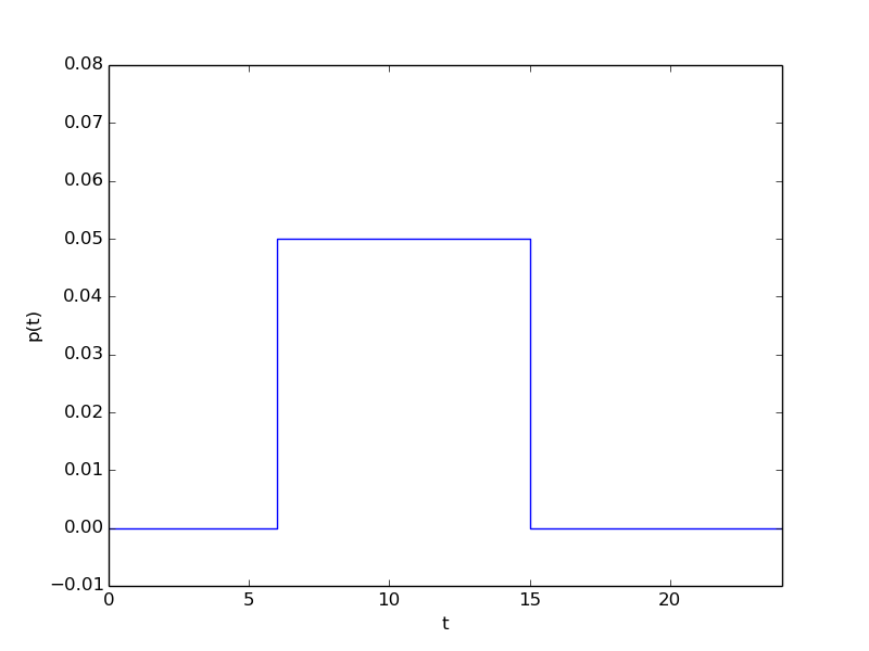
10 times more intense vaccination for 10 days, 6 days after outbreak:
$$
\begin{equation*} p(t) = \left\lbrace\begin{array}{ll}
0.005,& 6\leq t\leq 15,\\
0,& \hbox{otherwise} \end{array}\right.\end{equation*}
$$
Implementation: Let \( p^n \) be an array as \( V^n \). Set \( p^n=0.05 \) for \( n=6\cdot 24/0.1,\ldots, 15\cdot 24/0.1 \) (\( \mbox{days}\cdot 24 /\Delta t \), 24 is hours per day).
Effect of vaccination campaign
Note:
- Mathematicians would be scared by the cusps on the curves...
- Could now let the computer run a lot of cases and find the optimal vaccination period
We can experiment with other campaigns
|
|
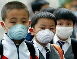
Wearing masks lowers \( \beta \):
Very easy to implement. (Used to be complicated in differential equation models...) |
And now for something similar: zombification!

Zombification: The disease that turns you into a zombie.
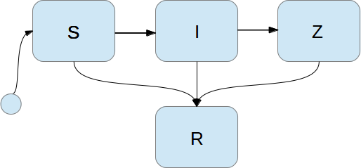
Zombie modeling is almost the same as SIR modeling
- S: susceptible humans who can become zombies
- I: infected humans, being bitten by zombies
- Z: zombies
- R: removed individuals, either conquered zombies or dead humans
Mathematical quantities: \( S(t) \), \( I(t) \), \( Z(t) \), \( R(t) \)
Zombie movie: The Night of the Living Dead, Geoerge A. Romero, 1968
Dynamics of the zombie SIZR model
- Susceptibles are infected by zombies: \( -\Delta t\beta SZ \) in time \( \Delta t \) (cf. the \( \Delta t\,\beta SI \) term in the SIR model).
- Susceptibles die naturally or get killed and then enter the removed category. The no of deaths in time \( \Delta t \) is \( \Delta t\delta_S S \).
- We also allow new humans to enter the area with zombies (necessary in a war on zombies): \( \Delta t\Sigma \) during a time \( \Delta t \).
- Some infected turn into zombies (Z): \( \Delta t\rho I \), while others die (R): \( \delta_I\Delta t I \).
- Nobody from R can turn into Z (important - otherwise zombies win).
- Killed zombies go to R: \( \Delta t\alpha SZ \).
The four equations in the SIZR model for zombification
$$
\begin{align*}
S^{n+1} &= S^n + \Delta t\,\Sigma - \Delta t\,\beta S^nZ - \Delta t\,\delta_S S^n\\
I^{n+1} &= I^n + \Delta t\,\beta S^nZ^n - \Delta t\,\rho I^n - \Delta t\,\delta_I I^n\\
Z^{n+1} &= Z^n + \Delta t\,\rho I^n - \Delta t\,\alpha S^nZ^n\\
R^{n+1} &= R^n + \Delta t\,\delta_S S^n + \Delta t\,\delta_I I^n +
\Delta t\,\alpha S^nZ^n
\end{align*}
$$
- \( \Sigma \): no of new humans brought into the zombified area per unit time.
- \( \beta \): the probability that a theoretically possible human-zombie pair actually meets physically, during a unit time interval, with the result that the human is infected.
- \( \delta_S \): the probability that a susceptible human is killed or dies, in a unit time interval.
- \( \delta_I \): the probability that an infected human is killed or dies, in a unit time interval.
- \( \rho \): the probability that an infected human is turned into a zombie, during a unit time interval.
- \( \alpha \): the probability that, during a unit time interval, a theoretically possible human-zombie pair fights and the human kills the zombie.
Simulate a zombie movie!
|
Three fundamental phases.
|
|
How do we do this? As \( p \) in the vaccination campaign - the parameters take on different constant values in different time intervals.
H. P. Langtangen, K.-A. Mardal and P. Røtnes: Escaping the Zombie Threat by Mathematics, in A. Whelan et al.: Zombies in the Academy - Living Death in Higher Education, University of Chicago Press, 2013
Effective war on zombies
Introduce attacks on zombies at selected times \( T_0, T_1, \ldots, T_m \).
Model: Replace \( \alpha \) by
$$ \alpha_0 + \omega (t),$$
where \( \alpha_0 \) is constant and \( \omega(t) \) is a series of
Gaussian functions (peaks) in time:
$$ \omega(t) = a\sum_{i=0}^m \exp{\left(-\frac{1}{2}\left({t - T_i\over\sigma}\right)\right)}
$$
Must experiment with values of \( a \) (strength), \( \sigma \) (duration is \( 6\sigma \)), point of attacks (\( T_i \)) - with proper values humans beat the zombies!
Summary
- A complex spreading of diseases can be modeled by intuitive, simple accounting of movement between categories
- Such models are knowns as compartment models
- Result: difference equations that are easy to simulate on a computer
- (Can let \( \Delta t\rightarrow 0 \) and get differential equations)
- Easy to add new effects (vaccination, campaigns, zombification)
Site: https://github.com/hplgit/disease-modeling. Just do
git clone https://github.com/hplgit/disease-modeling.git