$$ \newcommand{\tp}{\thinspace .} $$

Study guide: Software engineering with exponential decay models

Hans Petter Langtangen [1, 2]

[1] Center for Biomedical Computing, Simula Research Laboratory [2] Department of Informatics, University of Oslo

Feb 12, 2016

From flat program to module with functions

Mathematical model problem

$$ \begin{align*} u'(t) &= -au(t), \quad t \in (0,T]\\ u(0) &= I \end{align*} $$

Solution by $ \theta $-scheme:

$$ \begin{equation*} u^{n+1} = \frac{1 - (1-\theta) a\Delta t}{1 + \theta a\Delta t}u^n \end{equation*} $$

$ \theta =0 $: Forward Euler, $ \theta =1 $: Backward Euler, $ \theta =1/2 $: Crank-Nicolson (midpoint method)

Many will make a rough, flat program first

from numpy import *
from matplotlib.pyplot import *

A = 1
a = 2
T = 4
dt = 0.2
N = int(round(T/dt))
y = zeros(N+1)
t = linspace(0, T, N+1)
theta = 1
y[0] = A
for n in range(0, N):
    y[n+1] = (1 - (1-theta)*a*dt)/(1 + theta*dt*a)*y[n]

y_e = A*exp(-a*t) - y
error = y_e - y
E = sqrt(dt*sum(error**2))
print 'Norm of the error: %.3E' % E
plot(t, y, 'r--o')
t_e = linspace(0, T, 1001)
y_e = A*exp(-a*t_e)
plot(t_e, y_e, 'b-')
legend(['numerical, theta=%g' % theta, 'exact'])
xlabel('t')
ylabel('y')
show()

There are major issues with this solution

The notation in the program does not correspond exactly to the notation in the mathematical problem: the solution is called y and corresponds to $ u $ in the mathematical description, the variable A corresponds to the mathematical parameter $ I $, N in the program is called $ N_t $ in the mathematics.

There are no comments in the program.

New flat program

from numpy import *
from matplotlib.pyplot import *

I = 1
a = 2
T = 4
dt = 0.2
Nt = int(round(T/dt))     # no of time intervals
u = zeros(Nt+1)           # array of u[n] values
t = linspace(0, T, Nt+1)  # time mesh
theta = 1                 # Backward Euler method

u[0] = I                  # assign initial condition
for n in range(0, Nt):    # n=0,1,...,Nt-1
    u[n+1] = (1 - (1-theta)*a*dt)/(1 + theta*dt*a)*u[n]

# Compute norm of the error
u_e = I*exp(-a*t) - u     # exact u at the mesh points
error = u_e - u
E = sqrt(dt*sum(error**2))
print 'Norm of the error: %.3E' % E

# Compare numerical (u) and exact solution (u_e) in a plot
plot(t, u, 'r--o')
t_e = linspace(0, T, 1001)       # very fine mesh for u_e
u_e = I*exp(-a*t_e)
plot(t_e, u_e, 'b-')
legend(['numerical, theta=%g' % theta, 'exact'])
xlabel('t')
ylabel('u')
show()

Such flat programs are ideal for IPython notebooks!

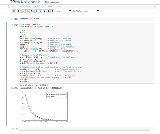
But: Further development of such flat programs require many scattered edits - easy to make mistakes!

The solution formula for $ u^{n+1} $ is completely general and should be available as a Python function with all input data as function arguments and all output data returned to the calling code

def solver(I, a, T, dt, theta):
    """Solve u'=-a*u, u(0)=I, for t in (0,T] with steps of dt."""
    dt = float(dt)               # avoid integer division
    Nt = int(round(T/dt))        # no of time intervals
    T = Nt*dt                    # adjust T to fit time step dt
    u = np.zeros(Nt+1)           # array of u[n] values
    t = np.linspace(0, T, Nt+1)  # time mesh

    u[0] = I                  # assign initial condition
    for n in range(0, Nt):    # n=0,1,...,Nt-1
        u[n+1] = (1 - (1-theta)*a*dt)/(1 + theta*dt*a)*u[n]
    return u, t

Call:

u, t = solver(I=1, a=2, T=4, dt=0.2, theta=0.5)

The DRY principle: Don't repeat yourself!

DRY:

When implementing a particular functionality in a computer program, make sure this functionality and its variations are implemented in just one piece of code. That is, if you need to revise the implementation, there should be one and only one place to edit. It follows that you should never duplicate code (don't repeat yourself!), and code snippets that are similar should be factored into one piece (function) and parameterized (by function arguments).

Make sure any program file is a valid Python module

Module requires code to be divided into functions :-)

Why module? Other programs can import the functions

from decay import solver
# Solve a decay problem
u, t = solver(I=1, a=2, T=4, dt=0.2, theta=0.5)

or prefix function names by the module name:

import decay
# Solve a decay problem
u, t = decay.solver(I=1, a=2, T=4, dt=0.2, theta=0.5)

The requirements of a module are so simple

The filename without .py must be a valid Python variable name.

The main program must be executed (through statements or a function call) in the test block.

The test block is normally placed at the end of a module file:

if __name__ == '__main__':
    # Statements

If the file is imported, the if test fails and no main program is run, otherwise, the file works as a program

The module file `decay.py` for our example

from numpy import *
from matplotlib.pyplot import *

def solver(I, a, T, dt, theta):
    ...

def u_exact(t, I, a):
    return I*exp(-a*t)

def experiment_compare_numerical_and_exact():
    I = 1;  a = 2;  T = 4;  dt = 0.4;  theta = 1
    u, t = solver(I, a, T, dt, theta)

    t_e = linspace(0, T, 1001)       # very fine mesh for u_e
    u_e = u_exact(t_e, I, a)

    plot(t,   u,   'r--o')           # dashed red line with circles
    plot(t_e, u_e, 'b-')             # blue line for u_e
    legend(['numerical, theta=%g' % theta, 'exact'])
    xlabel('t')
    ylabel('u')
    plotfile = 'tmp'
    savefig(plotfile + '.png');  savefig(plotfile + '.pdf')

    error = u_exact(t, I, a) - u
    E = sqrt(dt*sum(error**2))
    print 'Error norm:', E

if __name__ == '__main__':
    experiment_compare_numerical_and_exact()

Complete file: decay.py

The module file `decay.py` for our example w/prefix

import numpy as np
import matplotlib.pyplot as plt

def solver(I, a, T, dt, theta):
    ...

def u_exact(t, I, a):
    return I*np.exp(-a*t)

def experiment_compare_numerical_and_exact():
    I = 1;  a = 2;  T = 4;  dt = 0.4;  theta = 1
    u, t = solver(I, a, T, dt, theta)

    t_e = np.linspace(0, T, 1001)       # very fine mesh for u_e
    u_e = u_exact(t_e, I, a)

    plt.plot(t,   u,   'r--o')       # dashed red line with circles
    plt.plot(t_e, u_e, 'b-')         # blue line for u_e
    plt.legend(['numerical, theta=%g' % theta, 'exact'])
    plt.xlabel('t')
    plt.ylabel('u')
    plotfile = 'tmp'
    plt.savefig(plotfile + '.png');  plt.savefig(plotfile + '.pdf')

    error = u_exact(t, I, a) - u
    E = np.sqrt(dt*np.sum(error**2))
    print 'Error norm:', E

if __name__ == '__main__':
    experiment_compare_numerical_and_exact()

How do we add code for comparing schemes visually?

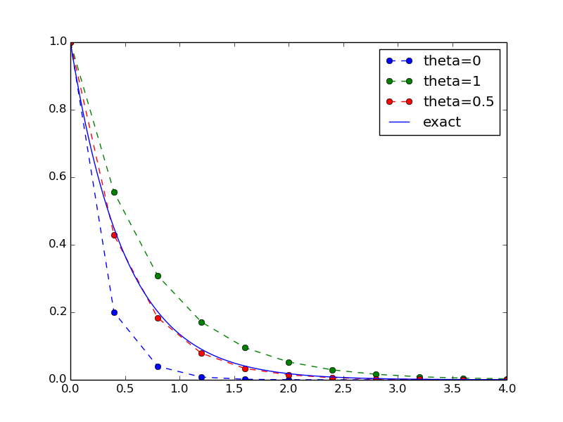
Think of edits in the flat program that are required to produce this plot (!)

We just add a new function with the tailored plotting

def experiment_compare_schemes():
    """Compare theta=0,1,0.5 in the same plot."""
    I = 1;  a = 2;  T = 4;  dt = 0.4
    legends = []
    for theta in [0, 1, 0.5]:
        u, t = solver(I, a, T, dt, theta)
        plt.plot(t, u, '--o')
        legends.append('theta=%g' % theta)
    t_e = np.linspace(0, T, 1001)        # very fine mesh for u_e
    u_e = u_exact(t_e, I, a)
    plt.plot(t_e, u_e, 'b-')
    legends.append('exact')
    plt.legend(legends, loc='upper right')
    plotfile = 'tmp'
    plt.savefig(plotfile + '.png');  plt.savefig(plotfile + '.pdf')

import logging
# Define a default logger that does nothing
logging.getLogger('decay').addHandler(logging.NullHandler())

def solver_with_logging(I, a, T, dt, theta):
    """Solve u'=-a*u, u(0)=I, for t in (0,T] with steps of dt."""
    dt = float(dt)               # avoid integer division
    Nt = int(round(T/dt))        # no of time intervals
    T = Nt*dt                    # adjust T to fit time step dt
    u = np.zeros(Nt+1)           # array of u[n] values
    t = np.linspace(0, T, Nt+1)  # time mesh
    logging.debug('solver: dt=%g, Nt=%g, T=%g' % (dt, Nt, T))

    u[0] = I                  # assign initial condition
    for n in range(0, Nt):    # n=0,1,...,Nt-1
        u[n+1] = (1 - (1-theta)*a*dt)/(1 + theta*dt*a)*u[n]

        logging.info('u[%d]=%g' % (n, u[n]))
        logging.debug('1 - (1-theta)*a*dt: %g, %s' %
                      (1-(1-theta)*a*dt,
                       str(type(1-(1-theta)*a*dt))[7:-2]))
        logging.debug('1 + theta*dt*a: %g, %s' %
                      (1 + theta*dt*a,
                       str(type(1 + theta*dt*a))[7:-2]))
    return u, t

def configure_basic_logger():
    logging.basicConfig(
        filename='decay.log', filemode='w', level=logging.DEBUG,
        format='%(asctime)s - %(levelname)s - %(message)s',
        datefmt='%Y.%m.%d %I:%M:%S %p')

The comparison

Prefixing imported functions by the module name

MATLAB-style names (linspace, plot):

from numpy import *
from matplotlib.pyplot import *

Python community convention is to prefix with module name (np.linspace, plt.plot):

import numpy as np
import matplotlib.pyplot as plt

Documenting functions and modules

Use NumPy-style doc strings!

See extensive documentation

These dominate in the Python scientific computing community

Easy to read with pydoc in the terminal

Can easily autogenerate beautiful online manuals

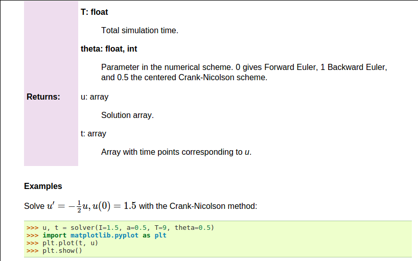
Example on NumPy-style doc string

def solver(I, a, T, dt, theta):
    """
    Solve :math:`u'=-au` with :math:`u(0)=I` for :math:`t \in (0,T]`
    with steps of `dt` and the method implied by `theta`.

    Parameters
    ----------
    I: float
        Initial condition.
    a: float
        Parameter in the differential equation.
    T: float
        Total simulation time.
    theta: float, int
        Parameter in the numerical scheme. 0 gives
        Forward Euler, 1 Backward Euler, and 0.5
        the centered Crank-Nicolson scheme.

    Returns
    -------
    `u`: array
        Solution array.
    `t`: array
        Array with time points corresponding to `u`.

    Examples
    --------
    Solve :math:`u' = -\\frac{1}{2}u, u(0)=1.5`
    with the Crank-Nicolson method:

    >>> u, t = solver(I=1.5, a=0.5, T=9, theta=0.5)
    >>> import matplotlib.pyplot as plt
    >>> plt.plot(t, u)
    >>> plt.show()
    """

Example on an autogenerated nice HTML manual

Can use a premade script to use Sphinx to generate an API manual in (e.g.) HTML

Logging intermediate results

Simulation programs often have long CPU times

Desire 1: monitor intermediate results/progress

Desire 2: turn on more intermediate results for debugging or troubleshooting

Most programming languages has a logging object for this purpose:

Write messages to a log file

Classify messages as critical, warning, info, or debug

Set logging level to one of the four types of messages

Introductory example on using a logger

import logging
import logging
logging.basicConfig(
    filename='myprog.log', filemode='w', level=logging.WARNING,
    format='%(asctime)s - %(levelname)s - %(message)s',
    datefmt='%m/%d/%Y %I:%M:%S %p')
logging.info('Here is some general info.')
logging.warning('Here is a warning.')
logging.debug('Here is some debugging info.')
logging.critical('Dividing by zero!')
logging.error('Encountered an error.')

Output in myprog.log:

09/26/2015 09:25:10 AM - INFO - Here is some general info.
09/26/2015 09:25:10 AM - WARNING - Here is a warning.
09/26/2015 09:25:10 AM - CRITICAL - Dividing by zero!
09/26/2015 09:25:10 AM - ERROR - Encountered an error.

A message is tied to a level, and one can specify one many levels that get printed

Levels: critical, error, warning, info, debug

level=logging.CRITICAL: print critical messages

level=logging.ERROR: print critical and error messages

level=logging.WARNING: print critical, error, and warning messages

level=logging.INFO: print critical, error, warning, and info messages

level=logging.DEBUG: print critical, error, warning, info, and debug messages

Using a logger in our solver function

import logging
# Define a default logger that does nothing
logging.getLogger('decay').addHandler(logging.NullHandler())

def solver_with_logging(I, a, T, dt, theta):
    """Solve u'=-a*u, u(0)=I, for t in (0,T] with steps of dt."""
    dt = float(dt)               # avoid integer division
    Nt = int(round(T/dt))        # no of time intervals
    T = Nt*dt                    # adjust T to fit time step dt
    u = np.zeros(Nt+1)           # array of u[n] values
    t = np.linspace(0, T, Nt+1)  # time mesh
    logging.debug('solver: dt=%g, Nt=%g, T=%g' % (dt, Nt, T))

    u[0] = I                  # assign initial condition
    for n in range(0, Nt):    # n=0,1,...,Nt-1
        u[n+1] = (1 - (1-theta)*a*dt)/(1 + theta*dt*a)*u[n]

        logging.info('u[%d]=%g' % (n, u[n]))
        logging.debug('1 - (1-theta)*a*dt: %g, %s' %
                      (1-(1-theta)*a*dt,
                       str(type(1-(1-theta)*a*dt))[7:-2]))
        logging.debug('1 + theta*dt*a: %g, %s' %
                      (1 + theta*dt*a,
                       str(type(1 + theta*dt*a))[7:-2]))
    return u, t

def configure_basic_logger():
    logging.basicConfig(
        filename='decay.log', filemode='w', level=logging.DEBUG,
        format='%(asctime)s - %(levelname)s - %(message)s',
        datefmt='%Y.%m.%d %I:%M:%S %p')

Monitoring messages

One terminal window (1M steps!):

>>> import decay
>>> u, t = decay.solver_with_logging(I=1, a=0.5, T=10, \ 
           dt=0.5, theta=0.5)

Another terminal window:

Terminal> tail -f decay.log
2015.09.26 05:37:41 AM - INFO - u[0]=1
2015.09.26 05:37:41 AM - INFO - u[1]=0.777778
2015.09.26 05:37:41 AM - INFO - u[2]=0.604938
2015.09.26 05:37:41 AM - INFO - u[3]=0.470508
2015.09.26 05:37:41 AM - INFO - u[4]=0.36595
2015.09.26 05:37:41 AM - INFO - u[5]=0.284628

Or if level=logging.DEBUG:

Terminal> tail -f decay.log
2015.09.26 05:40:01 AM - DEBUG - solver: dt=0.5, Nt=20, T=10
2015.09.26 05:40:01 AM - INFO - u[0]=1
2015.09.26 05:40:01 AM - DEBUG - 1 - (1-theta)*a*dt: 0.875, float
2015.09.26 05:40:01 AM - DEBUG - 1 + theta*dt*a: 1.125, float
2015.09.26 05:40:01 AM - INFO - u[1]=0.777778
2015.09.26 05:40:01 AM - DEBUG - 1 - (1-theta)*a*dt: 0.875, float
2015.09.26 05:40:01 AM - DEBUG - 1 + theta*dt*a: 1.125, float

User interfaces

Never edit the program to change input!

Set input data on the command line or in a graphical user interface

How is explained next

Accessing command-line arguments

All command-line arguments are available in sys.argv

sys.argv[0] is the program

sys.argv[1:] holds the command-line arguments

Method 1: fixed sequence of parameters on the command line

Method 2: --option value pairs on the command line (with default values)

Terminal> python myprog.py 1.5 2 0.5 0.8 0.4
Terminal> python myprog.py --I 1.5 --a 2 --dt 0.8 0.4

Reading a sequence of command-line arguments

Required input:

$ I $

$ a $

$ T $

name of scheme (FE, BE, CN)

a list of $ \Delta t $ values

Give these on the command line in correct sequence

Terminal> python decay_cml.py 1.5 0.5 4 CN 0.1 0.2 0.05

Implementation

def define_command_line_options():
    import argparse
    parser = argparse.ArgumentParser()
    parser.add_argument(
        '--I', '--initial_condition', type=float,
        default=1.0, help='initial condition, u(0)',
        metavar='I')
    parser.add_argument(
        '--a', type=float, default=1.0,
        help='coefficient in ODE', metavar='a')
    parser.add_argument(
        '--T', '--stop_time', type=float,
        default=1.0, help='end time of simulation',
        metavar='T')
    parser.add_argument(
        '--scheme', type=str, default='CN',
        help='FE, BE, or CN')
    parser.add_argument(
        '--dt', '--time_step_values', type=float,
        default=[1.0], help='time step values',
        metavar='dt', nargs='+', dest='dt_values')
    return parser

Note:

sys.argv[i] is always a string

Must explicitly convert to (e.g.) float for computations

List comprehensions make lists: [expression for e in somelist]

Working with an argument parser

Set option-value pairs on the command line if the default value is not suitable:

Terminal> python decay_argparse.py --I 1.5 --a 2 --dt 0.8 0.4

Code:

def read_command_line_argparse():
    parser = define_command_line_options()
    args = parser.parse_args()
    scheme2theta = {'BE': 1, 'CN': 0.5, 'FE': 0}
    data = (args.I, args.a, args.T, scheme2theta[args.scheme],
            args.dt_values)
    return data

(metavar is the symbol used in help output)

A graphical user interface

Normally very much programming required - and much competence on graphical user interfaces.

Here: use a tool to automatically create it in a few minutes (!)

The Parampool package

Parampool is a package for handling a large pool of input parameters in simulation programs

Parampool can automatically create a sophisticated web-based graphical user interface (GUI) to set parameters and view solutions

Remark.

The forthcoming material aims at those with particular interest in equipping their programs with a GUI - others can safely skip it.

Making a compute function

Key concept: a compute function that takes all input data as arguments and returning HTML code for viewing the results (e.g., plots and numbers)

What we have: decay_plot.py

main function carries out simulations and plotting for a series of $ \Delta t $ values

Goal: steer and view these experiments from a web GUI

What to do:

create a compute function

call parampool functionality

The compute function must return HTML code

def main_GUI(I=1.0, a=.2, T=4.0,
             dt_values=[1.25, 0.75, 0.5, 0.1],
             theta_values=[0, 0.5, 1]):
    # Build HTML code for web page. Arrange plots in columns
    # corresponding to the theta values, with dt down the rows
    theta2name = {0: 'FE', 1: 'BE', 0.5: 'CN'}
    html_text = '<table>\n'
    for dt in dt_values:
        html_text += '<tr>\n'
        for theta in theta_values:
            E, html = compute4web(I, a, T, dt, theta)
            html_text += """
<td>
<center><b>%s, dt=%g, error: %.3E</b></center><br>
%s
</td>
""" % (theta2name[theta], dt, E, html)
        html_text += '</tr>\n'
    html_text += '</table>\n'
    return html_text

Generating the user interface

Make a file decay_GUI_generate.py:

from parampool.generator.flask import generate
from decay import main_GUI
generate(main_GUI,
         filename_controller='decay_GUI_controller.py',
         filename_template='decay_GUI_view.py',
         filename_model='decay_GUI_model.py')

Running decay_GUI_generate.py results in

decay_GUI_model.py defines HTML widgets to be used to set input data in the web interface,

templates/decay_GUI_views.py defines the layout of the web page,

decay_GUI_controller.py runs the web application.

Good news: we only need to run decay_GUI_controller.py and there is no need to look into any of these files!

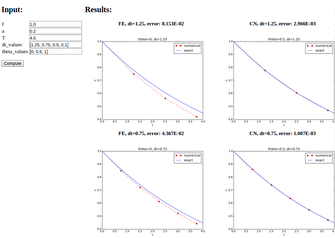
Running the web application

Start the GUI

Terminal> python decay_GUI_controller.py

Open a web browser at 127.0.0.1:5000

More advanced use

The compute function can have arguments of type float, int, string, list, dict, numpy array, filename (file upload)

Alternative: specify a hierarchy of input parameters with name, default value, data type, widget type, unit (m, kg, s), validity check

The generated web GUI can have user accounts with login and storage of results in a database

Tests for verifying implementations

Doctests

Doc strings can be equipped with interactive Python sessions for demonstrating usage and automatic testing of functions.

def solver(I, a, T, dt, theta):
    """
    Solve u'=-a*u, u(0)=I, for t in (0,T] with steps of dt.


    >>> u, t = solver(I=0.8, a=1.2, T=2, dt=0.5, theta=0.5)
    >>> for t_n, u_n in zip(t, u):
    ...     print 't=%.1f, u=%.14f' % (t_n, u_n)
    t=0.0, u=0.80000000000000
    t=0.5, u=0.43076923076923
    t=1.0, u=0.23195266272189
    t=1.5, u=0.12489758761948
    t=2.0, u=0.06725254717972
    """
    ...

Running doctests

Automatic check that the code reproduces the doctest output:

Terminal> python -m doctest decay.py

Floats are difficult to compare.

Limit the number of digits in the output in doctests! Otherwise, round-off errors on a different machine may ruin the test.

Unit testing with nose

Nose and pytest are a very user-friendly testing frameworks

Based on unit testing

Identify (small) units of code and test each unit

Nose automates running all tests

Good habit: run all tests after (small) edits of a code

Even better habit: write tests before the code (!)

Remark: unit testing in scientific computing is not yet well established

Basic use of nose and pytest

Implement tests in test functions with names starting with test_.

Test functions cannot have arguments.

Test functions perform assertions on computed results using assert functions from the nose.tools module.

Test functions can be in the source code files or be collected in separate files test*.py.

Example on a test function in the source code

Very simple module mymod (in file mymod.py):

def double(n):
    return 2*n

Write test function in mymod.py:

def double(n):
    return 2*n

def test_double():
    n = 4
    expected = 2*4
    computed = double(n)
    assert expected == computed

Running one of

Terminal> nosetests -s -v mymod
Terminal> py.test   -s -v mymod

makes the framework run all test_*() functions in mymod.py.

Example on test functions in a separate file

Write the test in a separate file, say test_mymod.py:

import mymod

def test_double():
    n = 4
    expected = 2*4
    computed = double(n)
    assert expected == computed

Running one of

Terminal> nosetests -s -v
Terminal> py.test   -s -v

makes the frameworks run all test_*() functions in all files test*.py in the current directory and in all subdirectories (pytest) or just those with names tests or *_tests (nose)

Tip.

Start with test functions in the source code file. When the file contains many tests, or when you have many source code files, move tests to separate files.

Test function for solver

Use exact discrete solution of the $ \theta $ scheme as test:

$$ u^n = I\left( \frac{1 - (1-\theta) a\Delta t}{1 + \theta a \Delta t} \right)^n$$

def u_discrete_exact(n, I, a, theta, dt):
    """Return exact discrete solution of the numerical schemes."""
    dt = float(dt)  # avoid integer division
    A = (1 - (1-theta)*a*dt)/(1 + theta*dt*a)
    return I*A**n

def test_u_discrete_exact():
    """Check that solver reproduces the exact discr. sol."""
    theta = 0.8; a = 2; I = 0.1; dt = 0.8
    Nt = int(8/dt)  # no of steps
    u, t = solver(I=I, a=a, T=Nt*dt, dt=dt, theta=theta)

    # Evaluate exact discrete solution on the mesh
    u_de = np.array([u_discrete_exact(n, I, a, theta, dt)
                     for n in range(Nt+1)])

    # Find largest deviation
    diff = np.abs(u_de - u).max()
    tol = 1E-14
    success = diff < tol
    assert success

Can test that potential integer division is avoided too

Warning.

If $ a $, $ \Delta t $, and $ \theta $ are integers, the formula for $ u^{n+1} $ in the solver function may lead to 0 because of unintended integer division.

def test_potential_integer_division():
    """Choose variables that can trigger integer division."""
    theta = 1; a = 1; I = 1; dt = 2
    Nt = 4
    u, t = solver(I=I, a=a, T=Nt*dt, dt=dt, theta=theta)
    u_de = np.array([u_discrete_exact(n, I, a, theta, dt)
                     for n in range(Nt+1)])
    diff = np.abs(u_de - u).max()
    assert diff < 1E-14

Packaging the software for other users

Python convention: install your software with setup.py

Installation of a single module file decay.py:

from distutils.core import setup
setup(name='decay',
      version='0.1',
      py_modules=['decay'],
      scripts=['decay.py'],
      )

Installation:

Terminal> sudo python setup.py install

(Many variants!)

split.py for several modules in a package

Python package = several modules

Modules be in a directory with a __init__.py file

Name of package = name of directory

setup.py:

from distutils.core import setup
import os

setup(name='decay',
      version='0.1',
      author='Hans Petter Langtangen',
      author_email='hpl@simula.no',
      url='https://github.com/hplgit/decay-package/',
      packages=['decay'],
      scripts=[os.path.join('decay', 'decay.py')]
     )

The `init.py` file can be empty

Empty __init__.py:

import decay
u, t = decay.decay.solver(...)

Do this in __init__.py to avoid decay.decay.solver:

from decay import *

Can now write

import decay
u, t = decay.solver(...)

# or
from decay import solver
u, t = solver(...)

Always develop software and write reports with Git

Git keeps track of different versions of files

Can roll back to previous versions

Can see who did what when

Can merge simultaneous edits by different users

Professionals rely on Git!

The Git work cycle:

git pull                # before starting a new session
# edit files
git add mynewfile       # remember to add new files!
git commit -am 'Short description of what I did'
git push origin master  # before end of day or a break

More pro use with Git

See what others have done in the project:

git fetch origin         # instead of git pull
git diff origin/master   # what are the changes?
git merge origin/master  # update my files

Develop new features in a separate branch:

git branch newstuff
git checkout newstuff
# edit files
git commit -am 'Changed ...'
git push origin newstuff

When newstuff is tested and matured, merge back in master:

git checkout master
git merge newstuff

Classes for problem and solution method

Collect physical problem and parameters in class Problem

from numpy import exp

class Problem(object):
    def __init__(self, I=1, a=1, T=10):
        self.T, self.I, self.a = I, float(a), T

    def u_exact(self, t):
        I, a = self.I, self.a
        return I*exp(-a*t)

Collect numerical parameters and methods in class Solver

class Solver(object):
    def __init__(self, problem, dt=0.1, theta=0.5):
        self.problem = problem
        self.dt, self.theta = float(dt), theta

    def solve(self):
        self.u, self.t = solver(
            self.problem.I, self.problem.a, self.problem.T,
            self.dt, self.theta)

    def error(self):
        """Return norm of error at the mesh points."""
        u_e = self.problem.u_exact(self.t)
        e = u_e - self.u
        E = np.sqrt(self.dt*np.sum(e**2))
        return E

Get input from the command line; class Problem

class Problem(object):
    def __init__(self, I=1, a=1, T=10):
        self.T, self.I, self.a = I, float(a), T

    def define_command_line_options(self, parser=None):
        """Return updated (parser) or new ArgumentParser object."""
        if parser is None:
            import argparse
            parser = argparse.ArgumentParser()

        parser.add_argument(
            '--I', '--initial_condition', type=float,
            default=1.0, help='initial condition, u(0)',
            metavar='I')
        parser.add_argument(
            '--a', type=float, default=1.0,
            help='coefficient in ODE', metavar='a')
        parser.add_argument(
            '--T', '--stop_time', type=float,
            default=1.0, help='end time of simulation',
            metavar='T')
        return parser

    def init_from_command_line(self, args):
        """Load attributes from ArgumentParser into instance."""
        self.I, self.a, self.T = args.I, args.a, args.T

Get input from the command line; class Problem

class Solver(object):
    def __init__(self, problem, dt=0.1, theta=0.5):
        self.problem = problem
        self.dt, self.theta = float(dt), theta

    def define_command_line_options(self, parser):
        """Return updated (parser) or new ArgumentParser object."""
        parser.add_argument(
            '--scheme', type=str, default='CN',
            help='FE, BE, or CN')
        parser.add_argument(
            '--dt', '--time_step_values', type=float,
            default=[1.0], help='time step values',
            metavar='dt', nargs='+', dest='dt_values')
        return parser

    def init_from_command_line(self, args):
        """Load attributes from ArgumentParser into instance."""
        self.dt, self.theta = args.dt, args.theta

How to combine class Problem and class Solver

def experiment_classes():
    problem = Problem()
    solver = Solver(problem)

    # Read input from the command line
    parser = problem.define_command_line_options()
    parser = solver. define_command_line_options(parser)
    args = parser.parse_args()
    problem.init_from_command_line(args)
    solver. init_from_command_line(args)

    # Solve and plot
    solver.solve()
    import matplotlib.pyplot as plt
    t_e = np.linspace(0, T, 1001)    # very fine mesh for u_e
    u_e = problem.u_exact(t_e)

    plt.plot(t,   u,   'r--o')       # dashed red line with circles
    plt.plot(t_e, u_e, 'b-')         # blue line for u_e
    plt.legend(['numerical, theta=%g' % theta, 'exact'])
    plt.xlabel('t')
    plt.ylabel('u')
    plt.show()

Performning scientific experiments

Goals:

Explore the behavior of a numerical method for an ODE

Show how a program can set up, execute, and report scientific investigations

Demonstrate how to write a scientific report

Demonstrate various technologies for reports: HTML w/MathJax, LaTeX, Sphinx, IPython notebooks, ...

Model problem and numerical solution method

Problem:

$$ \begin{equation} u'(t) = -au(t),\quad u(0)=I,\ 0 < t \leq T, \tag{1} \end{equation} $$

Solution method ($ \theta $-rule):

$$ u^{n+1} = \frac{1 - (1-\theta) a\Delta t}{1 + \theta a\Delta t}u^n, \quad u^0=I\tp $$

Plan for the experiments

For fixed $ I $, $ a $, and $ T $, we run the three schemes for various values of $ \Delta t $, and present in a report the following results:

visual comparison of the numerical and exact solution in a plot for each $ \Delta t $ and $ \theta=0,1,\frac{1}{2} $,

a table and a plot of the norm of the numerical error versus $ \Delta t $ for $ \theta=0,1,\frac{1}{2} $.

Available software

model.py:

Terminal> python model.py --I 1.5 --a 0.25 --T 6 --dt 1.25 0.75 0.5
0.0   1.25:    5.998E-01
0.0   0.75:    1.926E-01
0.0   0.50:    1.123E-01
0.0   0.10:    1.558E-02
0.5   1.25:    6.231E-02
0.5   0.75:    1.543E-02
0.5   0.50:    7.237E-03
0.5   0.10:    2.469E-04
1.0   1.25:    1.766E-01
1.0   0.75:    8.579E-02
1.0   0.50:    6.884E-02
1.0   0.10:    1.411E-02

+ a set of plot files of numerial vs exact solution

Required new results

Put plots together in table of plots

Table of numerical error vs $ \Delta t $ and $ \theta $

Log-log convergence plot of numerical error vs $ \Delta t $ for $ \theta=0,1,0.5 $

Must write a script exper1.py to automate running model.py and generating these results

Terminal> python exper1.py 0.5 0.25 0.1 0.05

($ \Delta t $ values on the comand line)

Reproducible science is key!

Let your scientific investigations be automated by scripts!

Excellent documentation

Trivial to re-run experiments

Easy to extend investigations

What actions are needed in the script?

Run model.py program with appropriate input

Interpret the output and make table and plot of numerical errors

Combine plot files to new figures

Complete script: exper1.py

Run a program from a program with `subprocess`

Command to be run:

python model.py --I 1.2 --a 0.2 --T 8 -dt 1.25 0.75 0.5 0.1

Constructed in Python:

# Given I, a, T, and a list dt_values
cmd = 'python model.py --I %g --a %g --T %g' % (I, a, T)
dt_values_str = ' '.join([str(v) for v in dt_values])
cmd += ' --dt %s' % dt_values_str

Run under the operating system:

from subprocess import Popen, PIPE, STDOUT
p = Popen(cmd, shell=True, stdout=PIPE, stderr=STDOUT)
output, dummy = p.communicate()

failure = p.returncode
if failure:
    print 'Command failed:', cmd; sys.exit(1)

Interpreting the output from an operating system command

The output if the previous command run by subprocess is in a string output:

errors = {'dt': dt_values, 1: [], 0: [], 0.5: []}
for line in output.splitlines():
    words = line.split()
    if words[0] in ('0.0', '0.5', '1.0'):  # line with E?
        # typical line: 0.0   1.25:    7.463E+00
        theta = float(words[0])
        E = float(words[2])
        errors[theta].append(E)

Combining plot files: PNG and PDF solutions

PNG:

Terminal> montage -background white -geometry 100% -tile 2x \ 
          f1.png f2.png f3.png f4.png f.png
Terminal> convert -trim f.png f.png
Terminal> convert f.png -transparent white f.png

PDF:

Terminal> pdftk f1.pdf f2.pdf f3.pdf f4.pdf output tmp.pdf
Terminal> pdfnup --nup 2x2 --outfile tmp.pdf tmp.pdf
Terminal> pdfcrop tmp.pdf f.pdf
Terminal> rm -f tmp.pdf

Easy to build these commands in Python and execute them with subprocess or os.system: os.system(cmd)

Making a report

Scientific investigations are best documented in a report!

A sample report

How can we write such a report?

First problem: what format should I write in?

Plain HTML

HTML with MathJax

LaTeX PDF, based on LaTeX source

Sphinx HTML, based on reStructuredText

IPython notebook, Markdown, MediaWiki, ...

DocOnce can generate LaTeX, HTML w/MathJax, Sphinx, IPython notebook, Markdown, MediaWiki, ... (DocOnce source for the examples above)

Examples on different report formats

Publishing a complete project

Make folder (directory) tree

Keep track of all files via a version control system (Git!)

Publish as private or public repository

Utilize Bitbucket or GitHub

See the intro to project hosting sites with version control

Study guide: Software engineering with exponential decay models

Feb 12, 2016

From flat program to module with functions

Mathematical model problem

Many will make a rough, flat program first

There are major issues with this solution

New flat program

Such flat programs are ideal for IPython notebooks!

But: Further development of such flat programs require many scattered edits - easy to make mistakes!

The DRY principle: Don't repeat yourself!

Make sure any program file is a valid Python module

The requirements of a module are so simple

The module file decay.py for our example

The module file decay.py for our example w/prefix

How do we add code for comparing schemes visually?

We just add a new function with the tailored plotting

The comparison

Prefixing imported functions by the module name

Documenting functions and modules

Example on NumPy-style doc string

Example on an autogenerated nice HTML manual

Logging intermediate results

Introductory example on using a logger

A message is tied to a level, and one can specify one many levels that get printed

Using a logger in our solver function

Monitoring messages

User interfaces

Accessing command-line arguments

Reading a sequence of command-line arguments

Implementation

Working with an argument parser

A graphical user interface

The Parampool package

Making a compute function

The compute function must return HTML code

Generating the user interface

Running the web application

More advanced use

Tests for verifying implementations

Doctests

Running doctests

Unit testing with nose

Basic use of nose and pytest

Example on a test function in the source code

Example on test functions in a separate file

Test function for solver

Can test that potential integer division is avoided too

Packaging the software for other users

Python convention: install your software with setup.py

split.py for several modules in a package

The __init__.py file can be empty

Always develop software and write reports with Git

More pro use with Git

Classes for problem and solution method

Collect physical problem and parameters in class Problem

Collect numerical parameters and methods in class Solver

Get input from the command line; class Problem

Get input from the command line; class Problem

How to combine class Problem and class Solver

Performning scientific experiments

Model problem and numerical solution method

Plan for the experiments

Available software

Required new results

Reproducible science is key!

What actions are needed in the script?

Run a program from a program with subprocess

Interpreting the output from an operating system command

Combining plot files: PNG and PDF solutions

Making a report

Publishing a complete project

The module file `decay.py` for our example

The module file `decay.py` for our example w/prefix

The `init.py` file can be empty

Run a program from a program with `subprocess`