A worked example on scientific computing with Python
Jan 20, 2015
Contents
This worked example
- fetches a data file from a web site,
- applies that file as input data for a differential equation modeling a vibrating mechanical system,
- solves the equation by a finite difference method,
- visualizes various properties of the solution and the input data.
The following programming topics are illustrated
- basic Python constructs: variables, loops, if-tests, arrays, functions
- flexible storage of objects in lists
- storage of objects in files (persistence)
- downloading files from the web
- user input via the command line
- signal processing and FFT
- curve plotting of data
- unit testing
- symbolic mathematics
- modules
All files can be forked at https://github.com/hplgit/bumpy
Table of contents
Contents
The following programming topics are illustrated
Scientific application
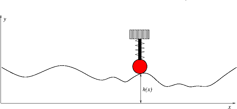
Physical problem and mathematical model
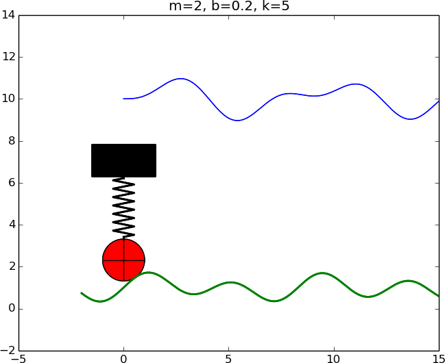
Relatively stiff spring \( k=5 \)
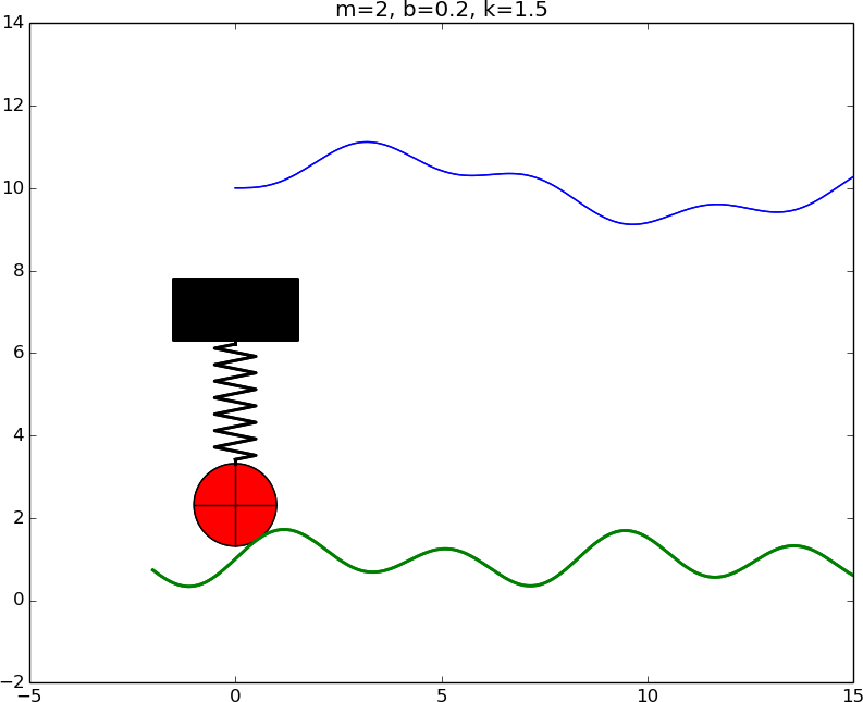
Softer spring \( k=1 \)
Numerical model
Extension to quadratic damping: \( f(u')=b|u'|u' \)
Simple implementation
Using the solver function to solve a problem
The resulting plot
More advanced implementation
The code (part I)
The code (part II)
Using the solver function to solve a problem
The resulting plot
Local vs global variables
Advanced programming of functions with parameters
The excitation force
The very basics of two-dimensional arrays
Computing the force from the road profile
Vectorized version of the previous function
Performing the simulation
A high-level solve function (part I)
A high-level solve function (part II)
Pickling: storing Python objects in files
Computing an expression for the noise level of the vibrations
User input
Positional command-line arguments
Option-value pairs on the command line
Example on using argparse
Running a simulation
Visual exploration
Code for loading data from file
Plotting the last part of \( u \)
Computing the derivative of \( u \)
Code for the derivative
How much faster is the vectorized version?
Computing the spectrum of signals
Plot of the spectra
Multiple plots in the same figure
Plot of the first realization
Advanced topics
Symbolic computing via SymPy
Go seamlessly from symbolic expression to Python function
Testing via test functions and test frameworks
Example on a test function
Test function for the numerical solver (part I)
Test function for the numerical solver (part II)
Test function for the numerical solver (part III)
Using a test framework
Modules
Example on a module file
What gets imported?
Scientific application

Physical problem and mathematical model
$$
\begin{equation}
mu'' + f(u') + s(u) = F(t),\quad u(0)=I,\ u'(0)=V
\tag{1}
\end{equation}
$$
- Input: mass \( m \), friction force \( f(u') \), spring \( s(u) \), external forcing \( F(t) \), \( I \), \( V \)
- Output: vertical displacement \( u(t) \)
Relatively stiff spring \( k=5 \)
Softer spring \( k=1 \)
Numerical model
- Finite difference method
- Centered differences
- \( u^n \): approximation to exact \( u \) at \( t=t_n=n\Delta t \)
- First: linear damping \( f(u')=bu' \)
$$
\begin{equation*}
u^{n+1} = \left(2mu^n + (\frac{b}{2}\Delta t - m)u^{n-1} +
\Delta t^2(F^n - s(u^n))
\right)(m + \frac{b}{2}\Delta t)^{-1}
\end{equation*}
$$
A special formula must be applied for \( n=0 \):
$$
\begin{equation*}
u^1 = u^0 + \Delta t\, V
+ \frac{\Delta t^2}{2m}(-bV - s(u^0) + F^0)
\end{equation*}
$$
Extension to quadratic damping: \( f(u')=b|u'|u' \)
Linearization via geometric mean:
$$
f(u'(t_n)) = \left. |u'|u'\right\vert^n \approx |u'|^{n-\frac{1}{2}}
(u')^{n+\frac{1}{2}}
$$
$$
\begin{align*}
u^{n+1} = & \left( m + b|u^n-u^{n-1}|\right)^{-1}\times \\
&\quad \left(2m u^n - mu^{n-1} + bu^n|u^n-u^{n-1}| + \Delta t^2 (F^n - s(u^n))
\right)
\end{align*}
$$
(and again a special formula for \( u^1 \))
Simple implementation
from numpy import *

def solver_linear_damping(I, V, m, b, s, F, t):
    N = t.size - 1              # No of time intervals
    dt = t[1] - t[0]            # Time step
    u = zeros(N+1)              # Result array
    u[0] = I
    u[1] = u[0] + dt*V + dt**2/(2*m)*(-b*V - s(u[0]) + F[0])

    for n in range(1,N):
        u[n+1] = 1./(m + b*dt/2)*(2*m*u[n] + \
                 (b*dt/2 - m)*u[n-1] + dt**2*(F[n] - s(u[n])))
    return u
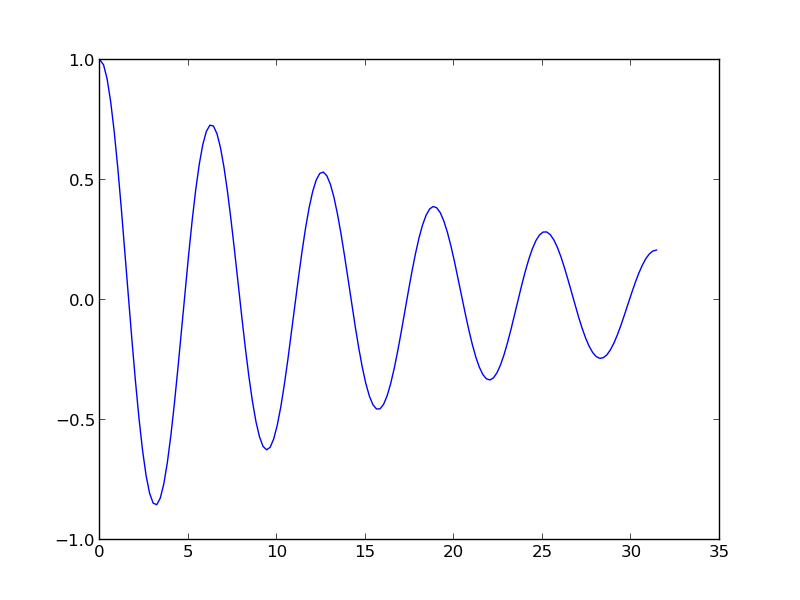
Using the solver function to solve a problem
from solver import solver_linear_damping
from numpy import *

def s(u):
    return 2*u

T = 10*pi      # simulate for t in [0,T]
dt = 0.2
N = int(round(T/dt))
t = linspace(0, T, N+1)
F = zeros(t.size)
I = 1; V = 0
m = 2; b = 0.2
u = solver_linear_damping(I, V, m, b, s, F, t)

from matplotlib.pyplot import *
plot(t, u)
savefig('tmp.pdf')   # save plot to PDF file
savefig('tmp.png')   # save plot to PNG file
show()
The resulting plot
More advanced implementation
Improvements:
- Treat linear and quadratic damping
- Allow \( F(t) \) to be either a function or an array of measurements
- Use doc strings for documentation
- Report errors through raising exceptions
- Watch out for integer division
>>> 2/3
0
>>> 2.0/3
0.6666666666666666
>>> 2/3.0
0.6666666666666666
At least one of the operands in division must be float
to get correct real division!
The code (part I)
def solver(I, V, m, b, s, F, t, damping='linear'):
    """
    Solve m*u'' + f(u') + s(u) = F for time points in t.
    u(0)=I and u'(0)=V,
    by a central finite difference method with time step dt.
    If damping is 'linear', f(u')=b*u, while if damping is
    'quadratic', we have f(u')=b*u'*abs(u').
    s(u) is a Python function, while F may be a function
    or an array (then F[i] corresponds to F at t[i]).
    """
    N = t.size - 1              # No of time intervals
    dt = t[1] - t[0]            # Time step
    u = np.zeros(N+1)           # Result array
    b = float(b); m = float(m)  # Avoid integer division

    # Convert F to array
    if callable(F):
        F = F(t)
    elif isinstance(F, (list,tuple,np.ndarray)):
        F = np.asarray(F)
    else:
        raise TypeError(
            'F must be function or array, not %s' % type(F))
The code (part II)
def solver(I, V, m, b, s, F, t, damping='linear'):
    ...
    u[0] = I
    if damping == 'linear':
        u[1] = u[0] + dt*V + dt**2/(2*m)*(-b*V - s(u[0]) + F[0])
    elif damping == 'quadratic':
        u[1] = u[0] + dt*V + \
               dt**2/(2*m)*(-b*V*abs(V) - s(u[0]) + F[0])
    else:
        raise ValueError('Wrong value: damping="%s"' % damping)

    for n in range(1,N):
        if damping == 'linear':
            u[n+1] = (2*m*u[n] + (b*dt/2 - m)*u[n-1] +
                      dt**2*(F[n] - s(u[n])))/(m + b*dt/2)
        elif damping == 'quadratic':
            u[n+1] = (2*m*u[n] - m*u[n-1] + b*u[n]*abs(u[n] - u[n-1])
                      - dt**2*(s(u[n]) - F[n]))/\
                      (m + b*abs(u[n] - u[n-1]))
    return u, t
Using the solver function to solve a problem
import numpy as np
from numpy import sin, pi # for nice math
from solver import solver
def F(t):
# Sinusoidal bumpy road
return A*sin(pi*t)
def s(u):
return k*(0.2*u + 1.5*u**3)
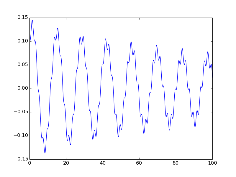
A = 0.25
k = 2
t = np.linspace(0, 100, 10001)
u, t = solver(I=0, V=0, m=2, b=0.5, s=s, F=F, t=t,
damping='quadratic')
# Show u(t) as a curve plot
import matplotlib.pyplot as plt
plt.plot(t, u)
plt.show()
The resulting plot
Local vs global variables
def f(u):
    return k*u
Here,
-
uis a local variable, which is accessible just inside in the function -
kis a global variable, which must be initialized outside the function prior to callingf
Advanced programming of functions with parameters
- \( f(u)=ku \) needs parameter \( k \)
- Implement \( f \) as a class with \( k \) as attribute and
__call__for evaluatingf(u)
class Spring:
    def __init__(self, k):
        self.k = k

    def __call__(self, u):
        return self.k*u

f = Spring(k)

# f looks like a function: can call f(0.2)
The excitation force
- A bumpy road gives an excitation \( F(t) \)
- File
bumpy.dat.gzcontains various road profiles \( h(x) \) - http://hplbit.bitbucket.org/data/bumpy/bumpy.dat.gz
Download road profile data \( h(x) \) from the Internet:
filename = 'bumpy.dat.gz'
url = 'http://hplbit.bitbucket.org/data/bumpy/bumpy.dat.gz'
import urllib
urllib.urlretrieve(url, filename)
h_data = np.loadtxt(filename)     # read numpy array from file

x = h_data[0,:]                # 1st column: x coordinates
h_data = h_data[1:,:]          # other columns: h shapes
The very basics of two-dimensional arrays
0     0.2   0.25  0.15
-0.1  0.15  0.2   0.15
>>> import numpy as np
>>> h_data = np.array([[0, 0.2, 0.25, 0.15],
                       [-0.1, 0.15, 0.2, 0.15]])
>>> h_data.shape  # size of each dimension
(2, 4)
>>> h_data[0,:]
array([ 0.  ,  0.2 ,  0.25,  0.15])
>>> h_data[:,0]
array([ 0. , -0.1])
>>> profile1 = h_data[1,:]
>>> profile1
array([-0.1 ,  0.15,  0.2 ,  0.15])
>>> h_data[1,1:3]                   # elements [1,1] [1,2]
array([ 0.15,  0.2 ])
Computing the force from the road profile
$$ F(t) \sim \frac{d^2}{dt^2}h(x),\ \ v=xt,\quad\Rightarrow\quad
F(t) \sim v^2 h''(x) $$
def acceleration(h, x, v):
    """Compute 2nd-order derivative of h."""
    # Method: standard finite difference aproximation
    d2h = np.zeros(h.size)
    dx = x[1] - x[0]
    for i in range(1, h.size-1, 1):
        d2h[i] = (h[i-1] - 2*h[i] + h[i+1])/dx**2
    # Extraplolate end values from first interior value
    d2h[0] = d2h[1]
    d2h[-1] = d2h[-2]
    a = d2h*v**2
    return a
Vectorized version of the previous function
def acceleration_vectorized(h, x, v):
    """Compute 2nd-order derivative of h. Vectorized version."""
    d2h = np.zeros(h.size)
    dx = x[1] - x[0]
    d2h[1:-1] = (h[:-2] - 2*h[1:-1] + h[2:])/dx**2
    # Extraplolate end values from first interior value
    d2h[0] = d2h[1]
    d2h[-1] = d2h[-2]
    a = d2h*v**2
    return a
Performing the simulation
Use a list data to hold all input and output data
data = [x, t]
for i in range(h_data.shape[0]):
    h = h_data[i,:]            # extract a column
    a = acceleration(h, x, v)
    F = -m*a
    u = solver(t=t, I=0, m=m, b=b, f=f, F=F)
    data.append([h, F, u])
Parameters for bicycle conditions: \( m=60 \) kg, \( v=5 \) m/s, \( k=60 \) N/m, \( b=80 \) Ns/m
A high-level solve function (part I)
def bumpy_road(url=None, m=60, b=80, k=60, v=5):
    """
    Simulate verticle vehicle vibrations.

    =========   ==============================================
    variable    description
    =========   ==============================================
    url         either URL of file with excitation force data,
                or name of a local file
    m           mass of system
    b           friction parameter
    k           spring parameter
    v           (constant) velocity of vehicle
    Return      data (list) holding input and output data
                [x, t, [h,F,u], [h,F,u], ...]
    =========   ==============================================
    """
    # Download file (if url is not the name of a local file)
    if url.startswith('http://') or url.startswith('file://'):
        import urllib
        filename = os.path.basename(url)  # strip off path
        urllib.urlretrieve(url, filename)
    else:
        # Check if url is the name of a local file
        if not os.path.isfile(url):
            print url, 'must be a URL or a filename'; sys.exit(1)
A high-level solve function (part II)
def bumpy_road(url=None, m=60, b=80, k=60, v=5):
    ...
    h_data = np.loadtxt(filename)  # read numpy array from file

    x = h_data[0,:]                # 1st column: x coordinates
    h_data = h_data[1:,:]          # other columns: h shapes

    t = x/v                        # time corresponding to x
    dt = t[1] - t[0]

    def f(u):
        return k*u

    data = [x, t]      # key input and output data (arrays)
    for i in range(h_data.shape[0]):
        h = h_data[i,:]            # extract a column
        a = acceleration(h, x, v)
	F = -m*a

        u = solver(t=t, I=0.2, m=m, b=b, f=f, F=F)

        data.append([h, F, u])
    return data
Pickling: storing Python objects in files
After calling
road_url = 'http://hplbit.bitbucket.org/data/bumpy/bumpy.dat.gz'
data = solve(url=road_url,
             m=60, b=200, k=60, v=6)
data = rms(data)
the data array contains single arrays and triplets of arrays,
[x, t, [h,F,u], [h,F,u], ..., [h,F,u]]
This list, or any Python object, can be stored on file for later retrieval of the results, using pickling:
import cPickle
outfile = open('bumpy.res', 'w')
cPickle.dump(data, outfile)
outfile.close()
Computing an expression for the noise level of the vibrations
$$ u_{\mbox{rms}} = \sqrt{T^{-1}\int_0^T u^2dt}
\approx \sqrt{\frac{1}{N+1}\sum_{i=0}^N (u^n)^2}$$
u_rms = []
for h, F, u in data[2:]:
    u_rms.append(np.sqrt((1./len(u))*np.sum(u**2))
Or by the more compact list comprehension:
u_rms = [np.sqrt((1./len(u))*np.sum(u**2))
         for h, F, u in data[2:]]
User input

Positional command-line arguments
Suppose \( b \) is given on the command line:
Terminal> python bumpy.py 10
Code:
try:
    b = float(sys.argv[1])
except IndexError:
    b = 80  # default
Note:
- Command-line arguments are in the list
sys.argv[1:] -
sys.argv[i]is a string, so float conversion is necessary before calculations
Option-value pairs on the command line
We can alternatively use option-value pairs on the command line:
Terminal> python bumpy.py --m 40 --b 280
Note:
- All parameters have default values
- The default value can be overridden on the command line with
--option value - We can use the
argparsemodule for defining, reading, and accessing option-value pairs
Example on using argparse
def command_line_options():
    import argparse
    parser = argparse.ArgumentParser()
    parser.add_argument('--m', '--mass', type=float,
                        default=60, help='mass of vehicle')
    parser.add_argument('--k', '--spring', type=float,
                        default=60, help='spring parameter')
    parser.add_argument('--b', '--damping', type=float,
                        default=80, help='damping parameter')
    parser.add_argument('--v', '--velocity', type=float,
                        default=5, help='velocity of vehicle')
    url = 'http://hplbit.bitbucket.org/data/bumpy/bumpy.dat.gz'
    parser.add_argument('--roadfile', type=str,
              default=url, help='filename/URL with road data')

    args = parser.parse_args()

    # Extract input parameters
    m = args.m; k = args.k; b = args.b; v = args.v
    url = args.roadfile
    return url, m, b, k, v
Running a simulation
Terminal> python bumpy.py --velocity 10
The rest of the parameters have their default values
Visual exploration
Plot
- \( u(t) \) and \( u'(t) \) for \( t\geq t_s \)
- the spectrum of \( u(t) \), for \( t\geq t_s \) (using FFT) to see which frequencies that dominate in the signal
- for each road shape, a plot of \( h(x) \), \( a(t) \), and \( u(t) \), for \( t \geq t_s \)
Code for loading data from file
Loading pickled results in file:
import cPickle
outfile = open('bumpy.res', 'r')
data = cPickle.load(outfile)
outfile.close()

x, t = data[0:2]
Recall list data:
[x, t, [h,F,u], [h,F,u], ..., [h,F,u]]
Further, for convenience (and Matlab-like code):
from numpy import *
from matplotlib.pyplot import *
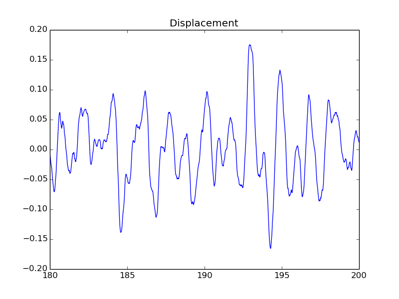
Plotting the last part of \( u \)
Display only the last portion of time series:
indices = t >= t_s   # True/False boolean array
t = t[indices]       # fetch the part of t for which t > t_s
x = x[indices]       # fetch the part of x for which t > t_s
Plotting \( u \):
figure()
realization = 1
u = data[2+realization][2][indices]
plot(t, u)
title('Displacement')
Note: data[2+realization] is a triplet [h,F,u]
Computing the derivative of \( u \)
$$
\begin{equation*}
v^n = \frac{u^{n+1}-u^{n-1}}{2\Delta t},\quad n=1,\ldots,N-1\thinspace .
\end{equation*}
$$
$$ v^0 = \frac{u^1-u^0}{\Delta t},\quad v^{N} = \frac{u^N-u^{N-1}}{\Delta t}$$
Code for the derivative
v = zeros_like(u)           # same length and data type as u
dt = t[1] - t[0]            # time step
for i in range(1,u.size-1):
    v[i] = (u[i+1] - u[i-1])/(2*dt)
v[0] = (u[1] - u[0])/dt
v[N] = (u[N] - u[N-1])/dt
Vectorized version:
v = zeros_like(u)

v[1:-1] = (u[2:] - u[:-2])/(2*dt)

v[0] = (u[1] - u[0])/dt
v[-1] = (u[-1] - u[-2])/dt
How much faster is the vectorized version?
IPython has the convenient %timeit feature for measuring CPU time:
In [1]: from numpy import zeros

In [2]: N = 1000000

In [3]: u = zeros(N)

In [4]: %timeit v = u[2:] - u[:-2]
1 loops, best of 3: 5.76 ms per loop

In [5]: v = zeros(N)

In [6]: %timeit for i in range(1,N-1): v[i] = u[i+1] - u[i-1]
1 loops, best of 3: 836 ms per loop

In [7]: 836/5.76
Out[20]: 145.13888888888889
145 times faster!
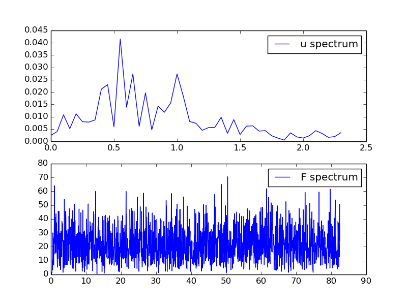
Computing the spectrum of signals
The spectrum of a discrete function \( u(t) \):
def frequency_analysis(u, t):
    A = fft(u)
    A = 2*A
    dt = t[1] - t[0]
    N = t.size
    freq = arange(N/2, dtype=float)/N/dt
    A = abs(A[0:freq.size])/N
    # Remove small high frequency part
    tol = 0.05*A.max()
    for i in xrange(len(A)-1, 0, -1):
        if A[i] > tol:
            break
    return freq[:i+1], A[:i+1]

figure()
u = data[3][2][indices]  # 2nd realization of u
f, A = frequency_analysis(u, t)
plot(f, A)
title('Spectrum of u')
Plot of the spectra
Multiple plots in the same figure
Run through all the 3-lists [h, F, u] and plot
these arrays:
for realization in range(len(data[2:])):
    h, F, u = data[2+realization]
    h = h[indices];  F = F[indices];  u = u[indices]

    figure()
    subplot(3, 1, 1)
    plot(x, h, 'g-')
    legend(['h %d' % realization])
    hmax = (abs(h.max()) + abs(h.min()))/2
    axis([x[0], x[-1], -hmax*5, hmax*5])
    xlabel('distance'); ylabel('height')

    subplot(3, 1, 2)
    plot(t, F)
    legend(['F %d' % realization])
    xlabel('t'); ylabel('acceleration')

    subplot(3, 1, 3)
    plot(t, u, 'r-')
    legend(['u %d' % realization])
    xlabel('t'); ylabel('displacement')
Plot of the first realization
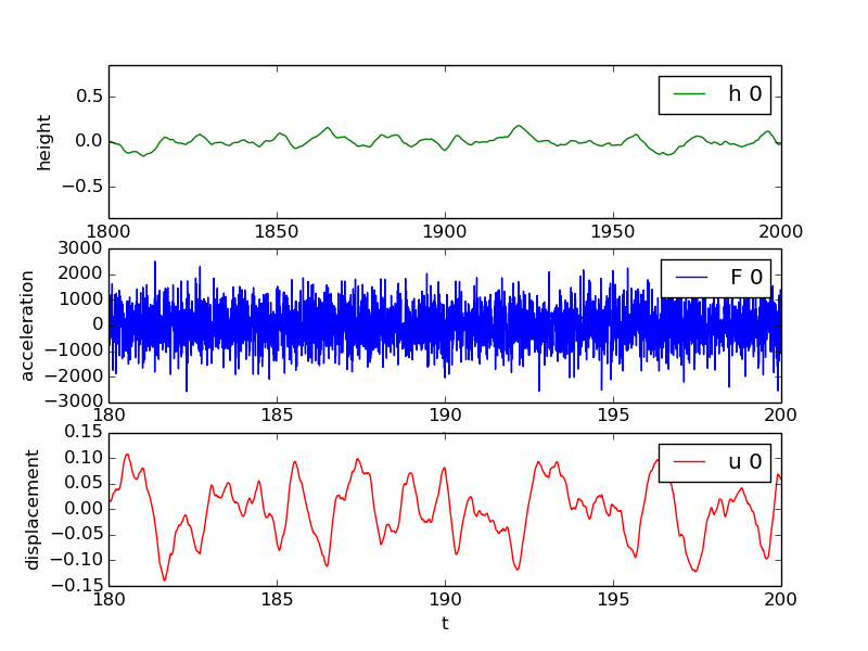
See explore.py
Advanced topics

Symbolic computing via SymPy
SymPy can do exact differentiation, integration, equation solving, ...
>>> import sympy as sp
>>> x, a = sp.symbols('x a')        # Define mathematical symbols
>>> Q = a*x**2 - 1                  # Quadratic function
>>> dQdx = sp.diff(Q, x)            # Differentiate wrt x
>>> dQdx
2*a*x
>>> Q2 = sp.integrate(dQdx, x)      # Integrate (no constant)
>>> Q2
a*x**2
>>> Q2 = sp.integrate(Q, (x, 0, a)) # Definite integral
>>> Q2
a**4/3 - a
>>> roots = sp.solve(Q, x)          # Solve Q = 0 wrt x
>>> roots
[-sqrt(1/a), sqrt(1/a)]
Go seamlessly from symbolic expression to Python function
Convert a SymPy expression Q into
a Python function Q(x, a):
>>> Q = sp.lambdify([x, a], Q)      # Turn Q into Py func.
>>> Q(x=2, a=3)                     # 3*2**2 - 1 = 11
11
This Q(x, a) function can be used for numerical computing
Testing via test functions and test frameworks
Modern test frameworks:
Use pytest, stay away from classical unittest
Example on a test function
def halve(x):
    """Return half of x."""
    return x/2.0

def test_halve():
    x = 4
    expected = 2
    computed = halve(x)
    # Compare real numbers using tolerance
    tol = 1E-14
    diff = abs(computed - expected)
    assert diff < tol
Note:
- Name starts with
test_* - No arguments
- Must have
asserton a boolean expression for passed test
Test function for the numerical solver (part I)
Show that \( u=I + Vt + qt^2 \) solves the discrete equations exactly for linear damping and with \( q=0 \) for quadratic damping
def lhs_eq(t, m, b, s, u, damping='linear'):
    """Return lhs of differential equation as sympy expression."""
    v = sm.diff(u, t)
    d = b*v if damping == 'linear' else b*v*sm.Abs(v)
    return m*sm.diff(u, t, t) + d + s(u)
Fit source term in differential equation to any chosen \( u(t) \):
t = sm.Symbol('t')
q = 2  # arbitrary constant
u_chosen = I + V*t + q*t**2   # sympy expression
F_term = lhs_eq(t, m, b, s, u_chosen, 'linear')
Test function for the numerical solver (part II)
import sympy as sm

def test_solver():
    """Verify linear/quadratic solution."""
    # Set input data for the test
    I = 1.2; V = 3; m = 2; b = 0.9; k = 4
    s = lambda u: k*u
    T = 2
    dt = 0.2
    N = int(round(T/dt))
    time_points = np.linspace(0, T, N+1)

    # Test linear damping
    t = sm.Symbol('t')
    q = 2  # arbitrary constant
    u_exact = I + V*t + q*t**2   # sympy expression
    F_term = lhs_eq(t, m, b, s, u_exact, 'linear')
    print 'Fitted source term, linear case:', F_term
    F = sm.lambdify([t], F_term)
    u, t_ = solver(I, V, m, b, s, F, time_points, 'linear')
    u_e = sm.lambdify([t], u_exact, modules='numpy')
    error = abs(u_e(t_) - u).max()
    tol = 1E-13
    assert error < tol
Test function for the numerical solver (part III)
def test_solver():
    ...
    # Test quadratic damping: u_exact must be linear
    u_exact = I + V*t
    F_term = lhs_eq(t, m, b, s, u_exact, 'quadratic')
    print 'Fitted source term, quadratic case:', F_term
    F = sm.lambdify([t], F_term)
    u, t_ = solver(I, V, m, b, s, F, time_points, 'quadratic')
    u_e = sm.lambdify([t], u_exact, modules='numpy')
    error = abs(u_e(t_) - u).max()
    assert error < tol
Using a test framework
Examine all subdirectories test* for test_*.py files:
Terminal> py.test -s
====================== test session starts =======================
...
collected 3 items

tests/test_bumpy.py .
Fitted source term, linear case: 8*t**2 + 15.6*t + 15.5
Fitted source term, quadratic case: 12*t + 12.9
testing solver
testing solver_linear_damping_wrapper

==================== 3 passed in 0.40 seconds ====================
Test a single file:
Terminal> py.test -s tests/test_bumpy.py
...
Modules
- Put functions in a file - that is a module
- Move main program to a function
- Use a test block for executable code (call to main function)
if __name__ == '__main__':
    <statements in the main program>
Example on a module file
import module1
from module2 import somefunc1, somefunc2

def myfunc1(...):
    ...

def myfunc2(...):
    ...

if __name__ == '__main__':
    <statements in the main program>
What gets imported?
Import everything from the previous module:
from mymod import *
This imports
-
module1,somefunc1,somefunc2(global names inmymod) -
myfunc1,myfunc2(global functions inmymod)