Appendix: Getting access to Python
This appendix describes different technologies for either installing Python on your own computer or accessing Python in the cloud. Plain Python is very easy to install and use in cloud services, but for this book we need many add-on packages for doing scientific computations. Python together with these packages constitute a complex software eco system that is non-trivial to build, so we strongly recommend to use one of the techniques described next [1].
| [1] | Some of the text is taken from the 4th edition of the book A Primer on Scientifi Programming with Python, by H. P. Langtangen, published by Springer, 2014. |
Required software
The strictly required software packages for working with this book are
- Python version 2.7 [Ref21]
- Numerical Python (NumPy) [Ref22] [Ref23] for array computing
- Matplotlib [Ref24] [Ref25] for plotting
Desired add-on packages are
- IPython [Ref26] [Ref27] for interactive computing
- SciTools [Ref28] for add-ons to NumPy
- ScientificPython [Ref29] for add-ons to NumPy
- pytest or nose for testing programs
- pip for installing Python packages
- Cython for compiling Python to C
- SymPy [Ref30] for symbolic mathematics
- SciPy [Ref31] for advanced scientific computing
Python 2 or 3
Python comes in two versions, version 2 and 3, and these are not
fully compatible. However, for the programs in this book, the differences
are very small,
the major one being print, which in Python 2 is a statement like
print 'a:', a, 'b:', b
while in Python 3 it is a function call
print( 'a:', a, 'b:', b)
The authors have written Python v2.7 code in this book in a way that
makes porting to version 3.4 or later trivial: most programs will just
need a fix of the print statement. This can be automatically done by
running 2to3 prog.py to transform a Python 2 program prog.py to
its Python 3 counterpart. One can also use tools like future or
six to easily write programs that run under both versions 2 and 3,
or the futurize program can automatically do this for you based on
v2.7 code.
Since many tools for doing scientific computing in Python are still only available for Python version 2, we use this version in the present book, but emphasize that it has to be v2.7 and not older versions.
There are different ways to get access to Python with the required packages:
- Use a computer system at an institution where the software is installed. Such a system can also be used from your local laptop through remote login over a network.
- Install the software on your own laptop.
- Use a web service.
A system administrator can take the list of software packages and install the missing ones on a computer system. For the two other options, detailed descriptions are given below.
Using a web service is very straightforward, but has the disadvantage that you are constrained by the packages that are allowed to install on the service. There are services at the time of this writing that suffice for working with most of this book, but if you are going to solve more complicated mathematical problems, you will need more sophisticated mathematical Python packages, more storage and more computer resources, and then you will benefit greatly from having Python installed on your own computer.
Anaconda and Spyder
Anaconda is a free Python distribution produced by Continuum Analytics and contains about 200 Python packages, as well as Python itself, for doing a wide range of scientific computations. Anaconda can be downloaded from http://continuum.io/downloads. Choose Python version 2.7.
The Integrated Development Environment (IDE) Spyder is included with Anaconda and is our recommended tool for writing and running Python programs on Mac and Windows, unless you have preference for a plain text editor for writing programs and a terminal window for running them.
Spyder on Mac
Spyder is started by typing spyder in a (new) Terminal application.
If you get an error message unknown locale, you need to type the
following line in the Terminal application, or preferably put the line
in your $HOME/.bashrc Unix initialization file:
export LANG=en_US.UTF-8; export LC_ALL=en_US.UTF-8
Installation of additional packages
Anaconda installs the pip tool that is handy to install additional
packages. In a Terminal application on Mac or in a PowerShell terminal
on Windows, write
pip install --user packagename
How to write and run a Python program
You have basically three choices to develop and test a Python program:
- use a text editor and a terminal window
- use an Integrated Development Environment (IDE), like Spyder, which offers a window with a text editor and functionality to run programs and observe the output
- use the IPython notebook
The IPython notebook is briefly descried in the section Writing IPython notebooks, while the other two options are outlined below.
The need for a text editor
Since programs consist of plain text, we need to write this text with the help of another program that can store the text in a file. You have most likely extensive experience with writing text on a computer, but for writing your own programs you need special programs, called editors, which preserve exactly the characters you type. The widespread word processors, Microsoft Word being a primary example, are aimed at producing nice-looking reports. These programs format the text and are not acceptable tools for writing your own programs, even though they can save the document in a pure text format. Spaces are often important in Python programs, and editors for plain text give you complete control of the spaces and all other characters in the program file.
Text editors
The most widely used editors for writing programs are Emacs and Vim, which are available on all major platforms. Some simpler alternatives for beginners are
- Linux: Gedit
- Mac OS X: TextWrangler
- Windows: Notepad++
We may mention that Python comes with an editor called Idle, which can be used to write programs on all three platforms, but running the program with command-line arguments is a bit complicated for beginners in Idle so Idle is not my favorite recommendation.
Gedit is a standard program on Linux platforms, but all other editors must be installed in your system. This is easy: just google the name, download the file, and follow the standard procedure for installation. All of the mentioned editors come with a graphical user interface that is intuitive to use, but the major popularity of Emacs and Vim is due to their rich set of short-keys so that you can avoid using the mouse and consequently edit at higher speed.
Terminal windows
To run the Python program, you need a terminal window. This is a
window where you can issue Unix commands in Linux and Mac OS X systems
and DOS commands in Windows. On a Linux computer, gnome-terminal
is my favorite, but other choices work equally well, such as xterm
and konsole. On a Mac computer, launch the application Utilities -
Terminal. On Windows, launch PowerShell.
You must first move to the right folder using the cd foldername
command. Then running a python program prog.py is a matter of
writing python prog.py. Whatever the program prints can be
seen in the terminal window.
Using a plain text editor and a terminal window
- Create a folder where your Python programs can be located, say
with name
mytestunder your home folder. This is most conveniently done in the terminal window since you need to use this window anyway to run the program. The command for creating a new folder ismkdir mytest. - Move to the new folder:
cd mytest. - Start the editor of your choice.
- Write a program in the editor, e.g., just the line
print 'Hello!'. Save the program under the namemyprog1.pyin themytestfolder. - Move to the terminal window and write
python myprog1.py. You should see the wordHello!being printed in the window.
Spyder
Spyder is a graphical application for developing and running Python
programs, available on all major platforms. Spyder comes with Anaconda
and some other pre-built environments for scientific computing with
Python. On Ubuntu it is conveniently installed by sudo apt-get
install spyder.
The left part of the Spyder window contains a plain text editor.
Click in this window and write print 'Hello!' and return.
Choose Run from the Run pull-down menu, and observe the output
Hello! in the lower right window where the output from
programs is visible.
You may continue with more advanced statements involving graphics:
import matplotlib.pyplot as plt
import numpy as np
x = np.linspace(0, 4, 101)
y = np.exp(-x)*np.sin(np.pi*x)
plt.plot(x,y)
plt.title('First test of Spyder')
plt.savefig('tmp.png')
plt.show()
Choosing Run - Run now leads to a separate window with a plot of the function \(e^{-x}\sin (\pi x)\). Figure The Spyder Integrated Development Environment shows how the Spyder application may look like.
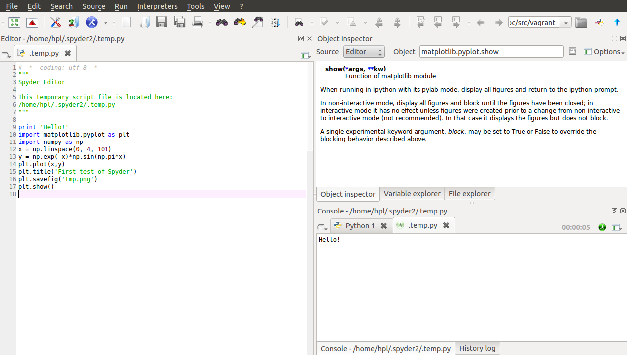
The Spyder Integrated Development Environment
The plot file we generate in the above program,
tmp.png, is by default found in the Spyder folder listed in
the default text in the top of the program. You can choose
Run - Configure ... to change this folder as desired.
The program you write is written to a file .temp.py in the same
default folder, but any name and folder can be specified in the
standard File - Save as... menu.
A convenient feature of Spyder is that the upper right window continuously displays documentation of the statements you write in the editor to the left.
The SageMathCloud and Wakari web services
You can avoid installing Python on your machine completely by using a web service that allows you to write and run Python programs. Computational science projects will normally require some kind of visualization and associated graphics packages, which is not possible unless the service offers IPython notebooks. There are two excellent web services with notebooks: SageMathCloud at https://cloud.sagemath.com/ and Wakari at https://www.wakari.io/wakari. At both sites you must create an account before you can write notebooks in the web browser and download them to your own computer.
Basic intro to SageMathCloud
Sign in, click on New Project, give a title to your project and
decide whether it should be private or public, click on the project
when it appears in the browser, and click on Create or Import a File,
Worksheet, Terminal or Directory.... If your Python program needs
graphics, you need to choose IPython Notebook, otherwise you can
choose File. Write the name of the file above the row of
buttons. Assuming we do not need any graphics, we create a plain Python
file, say with name
py1.py. By clicking File you are brought to a browser window with
a text editor where you can write Python code. Write some code and
click Save. To run the program, click on the plus icon (New),
choose Terminal, and you have a plain Unix terminal window where you
can write python py1.py to run the program. Tabs over the terminal
(or editor) window make it easy to jump between the editor and the
terminal. To download the file, click on Files, point on the
relevant line with the file, and a download icon appears to the very
right. The IPython notebook option works much in the same way, see
the section Writing IPython notebooks.
Basic intro to Wakari
After having logged in at the wakari.io site, you automatically
enter an IPython notebook with a short introduction to how the
notebook can be used. Click on the New Notebook button to start a
new notebook. Wakari enables creating and editing plain Python files too:
click on the Add file icon in pane to the left, fill in the program
name, and you enter an editor where you can write a program. Pressing
Execute launches an IPython session in a terminal window, where you
can run the program by run prog.py if prog.py is the name of the
program. To download the file, select test2.py in the left pane and
click on the Download file icon.
There is a pull-down menu where you can choose what type of terminal window you want: a plain Unix shell, an IPython shell, or an IPython shell with Matplotlib for plotting. Using the latter, you can run plain Python programs or commands with graphics. Just choose the type of terminal and click on +Tab to make a new terminal window of the chosen type.
Installing your own Python packages
Both SageMathCloud and Wakari let you install your own Python
packages.
To install any package packagename
available at PyPi, run
pip install --user packagename
To install the SciTools package, which is useful when working with this book, run the command
pip install --user -e \
    git+https://github.com/hplgit/scitools.git#egg=scitools
Writing IPython notebooks
The IPython notebook is a splendid interactive tool for doing science,
but it can also be used as a platform for developing Python code.
You can either run it locally on your computer or in a web service
like SageMathCloud or Wakari. Installation on your computer
is trivial on Ubuntu, just sudo apt-get install ipython-notebook, and
also on Windows and Mac by
using Anaconda or Enthought Canopy for the Python installation.
The interface to the notebook is a web browser: you write all the code and see all the results in the browser window. There are excellent YouTube videos on how to use the IPython notebook, so here we provide a very quick “step zero” to get anyone started.
A simple program in the notebook
Start the IPython notebook locally by the command ipython notebook
or go to SageMathCloud or Wakari as described above.
The default input area is a cell for Python code.
Type
g = 9.81
v0 = 5
t = 0.6
y = v0*t - 0.5*g*t**2
in a cell and run the cell by clicking on Run Selected (notebook running
locally on your machine)
or on the “play” button (notebook running in the cloud).
This action will execute the Python code and initialize the
variables g, v0, t, and y. You can then write print y in a
new cell, execute that cell, and see the output of this statement in
the browser. It is easy to go back to a cell, edit the code, and
re-execute it.
To download the notebook to your computer, choose the
File - Download as menu and select the type of file
to be downloaded: the original notebook format (.ipynb file
extension) or a plain Python program version of the notebook
(.py file extension).
Mixing text, mathematics, code, and graphics
The real strength of IPython notebooks arises when you want to write a report to document how a problem can be explored and solved. As a teaser, open a new notebook, click in the first cell, and choose Markdown as format (notebook running locally) or switch from Code to Markdown in the pull-down menu (notebook in the cloud). The cell is now a text field where you can write text with Markdown syntax. Mathematics can be entered as LaTeX code. Try some text with inline mathematics and an equation on a separate line:
Plot the curve $y=f(x)$, where

$$
f(x) = e^{-x}\sin (2\pi x),\quad x\in [0, 4]
$$
Execute the cell and you will see nicely typeset mathematics in the browser. In the new cell, add some code to plot \(f(x)\):
import numpy as np
import matplotlib.pyplot as plt
%matplotlib inline  # make plots inline in the notebook

x = np.linspace(0, 4, 101)
y = np.exp(-x)*np.sin(2*pi*x)
plt.plot(x, y, 'b-')
plt.xlabel('x'); plt.ylabel('y')
Executing these statements results in a plot in the browser, see
Figure Example on an IPython notebook. It was popular to
start the notebook by ipython notebook --pylab to import
everything from numpy and matplotlib.pyplot and make
all plots inline, but the --pylab option is now
officially discouraged.
If you want the notebook to behave more as MATLAB and not use
the np and plt prefix, you can instead of the first three
lines above write %pylab.
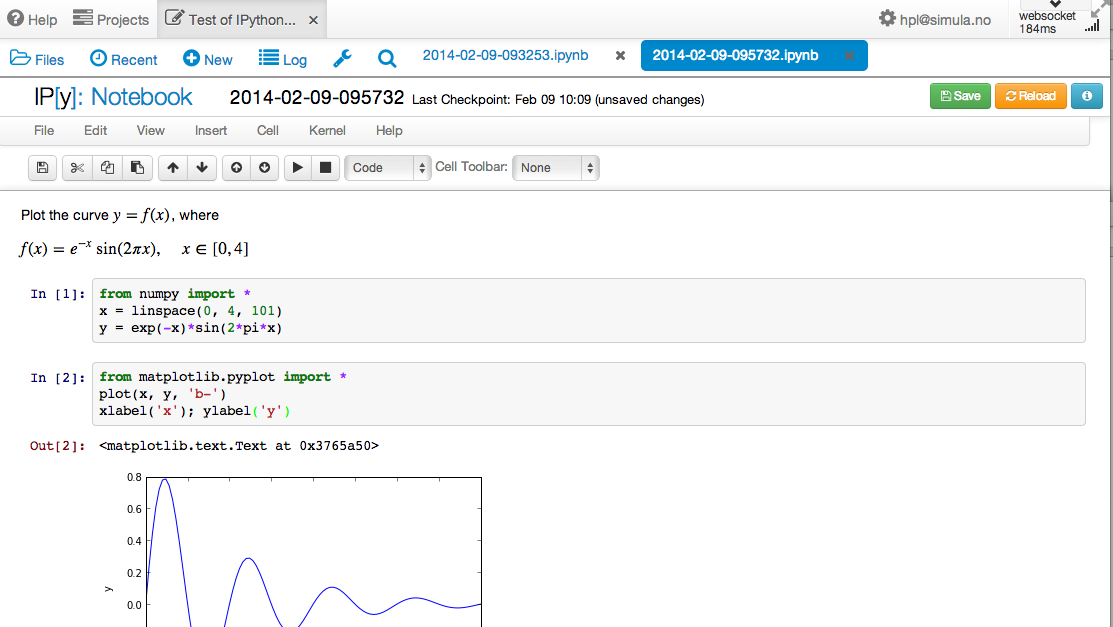
Example on an IPython notebook
