The IPython notebook is a splendid interactive tool for doing science,
but it can also be used as a platform for developing Python code.
You can either run it locally on your computer or in a web service
like SageMathCloud or Wakari. Installation on your computer
is trivial on Ubuntu, just sudo apt-get install ipython-notebook, and
also on Windows and Mac by
using Anaconda or Enthought Canopy for the Python installation.
The interface to the notebook is a web browser: you write all the code and see all the results in the browser window. There are excellent YouTube videos on how to use the IPython notebook, so here we provide a very quick "step zero" to get anyone started.
Start the IPython notebook locally by the command ipython notebook
or go to SageMathCloud or Wakari as described above.
The default input area is a cell for Python code.
Type
g = 9.81
v0 = 5
t = 0.6
y = v0*t - 0.5*g*t**2
g, v0, t, and y. You can then write print y in a
new cell, execute that cell, and see the output of this statement in
the browser. It is easy to go back to a cell, edit the code, and
re-execute it.
To download the notebook to your computer, choose the
File - Download as menu and select the type of file
to be downloaded: the original notebook format (.ipynb file
extension) or a plain Python program version of the notebook
(.py file extension).
The real strength of IPython notebooks arises when you want to write a report to document how a problem can be explored and solved. As a teaser, open a new notebook, click in the first cell, and choose Markdown as format (notebook running locally) or switch from Code to Markdown in the pull-down menu (notebook in the cloud). The cell is now a text field where you can write text with Markdown syntax. Mathematics can be entered as LaTeX code. Try some text with inline mathematics and an equation on a separate line:
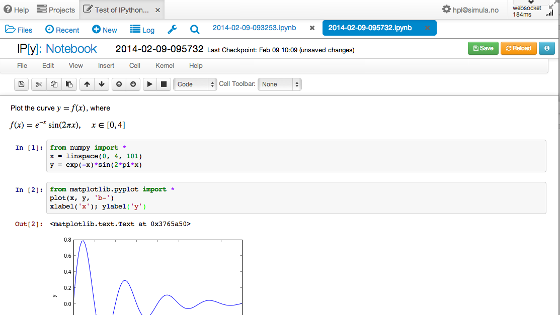
Plot the curve $y=f(x)$, where

$$
f(x) = e^{-x}\sin (2\pi x),\quad x\in [0, 4]
$$
from numpy import *
x = linspace(0, 4, 101)
y = exp(-x)*sin(2*pi*x)
from matplotlib.pyplot import *
plot(x, y, 'b-')
xlabel('x'); ylabel('y')
numpy and
matplotlib are imported by default when running the notebook
in the browser or by supplying the command-line argument --pylab
when starting notebooks locally on your machine.