$$
\newcommand{\Oof}[1]{\mathcal{O}(#1)}
\newcommand{\F}{\boldsymbol{F}}
\newcommand{\J}{\boldsymbol{J}}
\newcommand{\x}{\boldsymbol{x}}
\renewcommand{\c}{\boldsymbol{c}}
$$
The secant method
When finding the derivative \( f'(x) \) in Newton's method is problematic,
or when function evaluations take too long; we may adjust the method
slightly. Instead of using tangent lines to the graph we may use
secants.
The approach is referred to as the secant method, and the
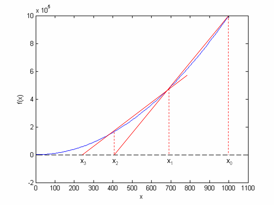
idea is illustrated graphically in Figure 63 for
our example problem \( x^2 - 9 = 0 \).
Figure 63: Illustrates the use of secants in the secant method when solving \( x^2 - 9 = 0, x \in [0, 1000] \). From two chosen starting values, \( x_0 = 1000 \) and \( x_1 = 700 \) the crossing \( x_2 \) of the corresponding secant with the \( x \) axis is computed, followed by a similar computation of \( x_3 \) from \( x_1 \) and \( x_2 \).

The idea of the secant method is to think as in Newton's method, but
instead of using \( f'(x_n) \), we approximate this derivative by a
finite difference or the secant, i.e., the slope of the straight
line that goes through the two most recent approximations \( x_n \) and
\( x_{n-1} \). This slope reads
$$
\begin{equation}
\frac{f(x_n)-f(x_{n-1})}{x_n - x_{n-1}}\thinspace .
\tag{153}
\end{equation}
$$
Inserting this expression for \( f'(x_n) \) in Newton's method simply gives
us the secant method:
$$
x_{n+1} = x_n - \frac{f(x_n)}{\frac{f(x_n)-f(x_{n-1})}{x_n - x_{n-1}}},$$
or
$$
\begin{equation}
x_{n+1} = x_n - f(x_n) \frac{x_n - x_{n-1}}{f(x_n)-f(x_{n-1})}
\thinspace .
\tag{154}
\end{equation}
$$
Comparing (154) to the graph in Figure
63, we see how two chosen starting points (\( x_0
= 1000 \), \( x_1= 700 \), and corresponding function values) are used to
compute \( x_2 \). Once we have \( x_2 \), we similarly use \( x_1 \) and \( x_2 \) to
compute \( x_3 \). As with Newton's method, the procedure is repeated
until \( f(x_n) \) is below some chosen limit value, or some limit on the
number of iterations has been reached. We use an iteration counter
here too, based on the same thinking as in the implementation of
Newton's method.
We can store the approximations \( x_n \) in an array, but as in Newton's
method, we notice that the computation of \( x_{n+1} \) only needs
knowledge of \( x_n \) and \( x_{n-1} \), not "older"
approximations. Therefore, we can make use of only three variables:
x for \( x_{n+1} \), x1 for \( x_n \), and x0 for \( x_{n-1} \). Note that
x0 and x1 must be given (guessed) for the algorithm to start.
A program
secant_method.py
that solves our example problem may be written as:
def secant(f, x0, x1, eps):
    f_x0 = f(x0)
    f_x1 = f(x1)
    iteration_counter = 0
    while abs(f_x1) > eps and iteration_counter < 100:
        try:
            denominator = float(f_x1 - f_x0)/(x1 - x0)
            x = x1 - float(f_x1)/denominator
        except ZeroDivisionError:
            print "Error! - denominator zero for x = ", x
            sys.exit(1)     # Abort with error
        x0 = x1
        x1 = x
        f_x0 = f_x1
        f_x1 = f(x1)
        iteration_counter += 1
    # Here, either a solution is found, or too many iterations
    if abs(f_x1) > eps:
        iteration_counter = -1
    return x, iteration_counter

def f(x):
    return x**2 - 9

x0 = 1000;   x1 = x0 - 1

solution, no_iterations = secant(f, x0, x1, eps=1.0e-6)

if no_iterations > 0:    # Solution found
    print "Number of function calls: %d" % (2 + no_iterations)
    print "A solution is: %f" % (solution)
else:
    print "Solution not found!"
The number of function calls is now related to no_iterations,
i.e., the number of iterations, as 2 + no_iterations, since we need
two function calls before entering the while loop, and then one
function call per loop iteration. Note that, even though we need two
points on the graph to compute each updated estimate, only a single
function call (f(x1)) is required in each iteration since
f(x0) becomes the "old" f(x1) and may simply be copied as
f_x0 = f_x1 (the exception is the very first iteration where two function
evaluations are needed).
Running secant_method.py, gives the following printout on the screen:
Number of function calls: 19
A solution is: 3.000000
As with the function Newton, we place secant in
the file nonlinear_solvers.py for easy import and use later.
