Experiments with Schemes for Exponential Decay¶

Author:	Hans Petter Langtangen (hpl at simula.no)
Date:	August 20, 2012

Summary. This report investigates the accuracy of three finite difference schemes for the ordinary differential equation \(u'=-au\) with the aid of numerical experiments. Numerical artifacts are in particular demonstrated.

Mathematical problem¶

We address the initial-value problem

\[\begin{split}u'(t) &= -au(t), \quad t \in (0,T], \\ u(0) &= I,\end{split}\]

where \(a\), \(I\), and \(T\) are prescribed parameters, and \(u(t)\) is the unknown function to be estimated. This mathematical model is relevant for physical phenomena featuring exponential decay in time.

Numerical solution method¶

We introduce a mesh in time with points \(0= t_0< t_1 \cdots < t_N=T\). For simplicity, we assume constant spacing \(\Delta t\) between the mesh points: \(\Delta t = t_{n}-t_{n-1}\), \(n=1,\ldots,N\). Let \(u^n\) be the numerical approximation to the exact solution at \(t_n\).

The \(\theta\)-rule is used to solve (ode) numerically:

\[u^{n+1} = \frac{1 - (1-\theta) a\Delta t}{1 + \theta a\Delta t}u^n,\]

for \(n=0,1,\ldots,N-1\). This scheme corresponds to

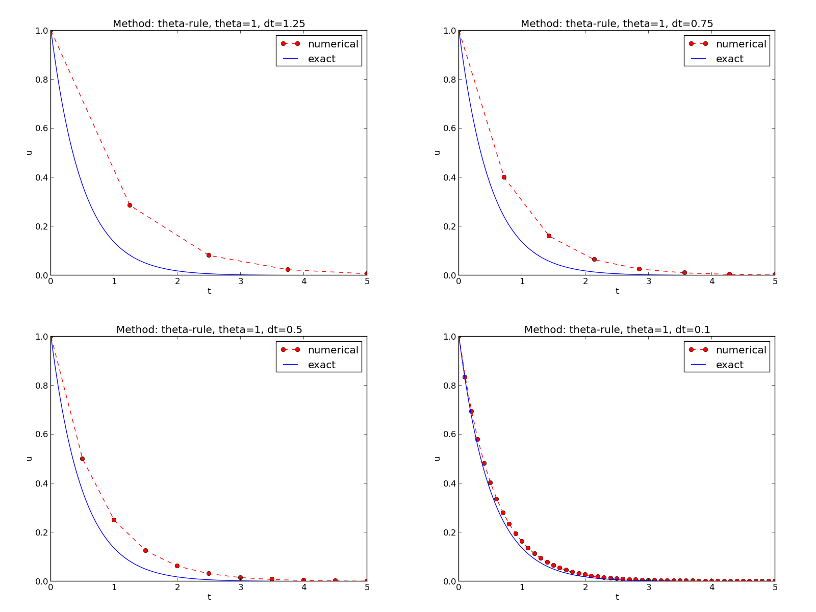
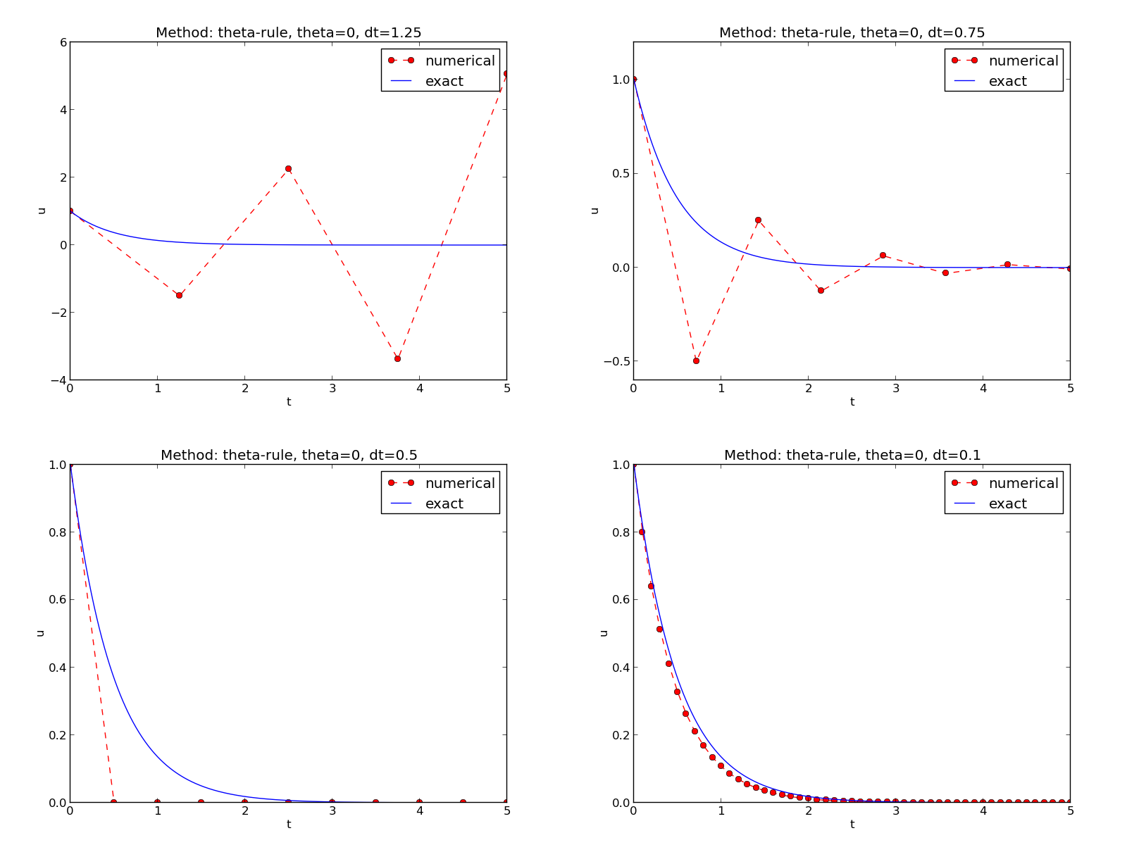
The Forward Euler scheme when \(\theta=0\)

The Backward Euler scheme when \(\theta=1\)

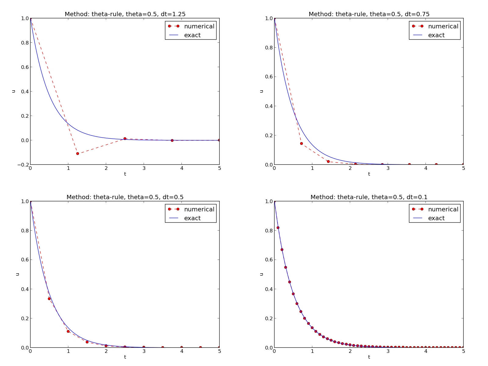
The Crank-Nicolson scheme when \(\theta=1/2\)

Implementation¶

The numerical method is implemented in a Python function:

def theta_rule(I, a, T, dt, theta):
    """Solve u'=-a*u, u(0)=I, for t in (0,T] with steps of dt."""
    N = int(round(T/float(dt)))  # no of intervals
    u = zeros(N+1)
    t = linspace(0, T, N+1)

    u[0] = I
    for n in range(0, N):
        u[n+1] = (1 - (1-theta)*a*dt)/(1 + theta*dt*a)*u[n]
    return u, t

Numerical experiments¶

We define a set of numerical experiments where \(I\), \(a\), and \(T\) are fixed, while \(\Delta t\) and \(\theta\) are varied. In particular, \(I=1\), \(a=2\), \(\Delta t = 1.25, 0.75, 0.5, 0.1\).

The Backward Euler method¶

The Crank-Nicolson method¶

The Forward Euler method¶

Error vs \(\Delta t\)¶

How \(E\) varies with \(\Delta t\) for \(\theta=0,0.5,1\) is shown in Figure Error versus time step.

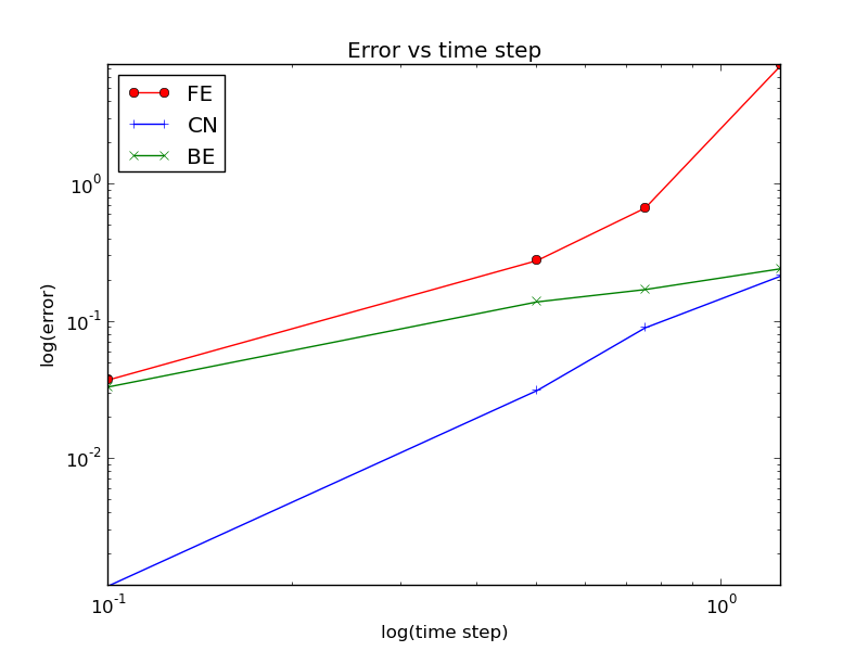
Error versus time step