Summary. This report investigates the accuracy of three finite difference schemes for the ordinary differential equation \( u'=-au \) with the aid of numerical experiments. Numerical artifacts are in particular demonstrated.
Mathematical problem
Numerical solution method
Implementation
Numerical experiments
The Backward Euler method
The Crank-Nicolson method
The Forward Euler method
Error vs \( \Delta t \)
We address the initial-value problem
$$ \begin{align} u'(t) &= -au(t), \quad t \in (0,T], \label{ode}\\ u(0) &= I, \label{initial:value} \end{align} $$ where \( a \), \( I \), and \( T \) are prescribed parameters, and \( u(t) \) is the unknown function to be estimated. This mathematical model is relevant for physical phenomena featuring exponential decay in time.
We introduce a mesh in time with points \( 0= t_0< t_1 \cdots < t_N=T \). For simplicity, we assume constant spacing \( \Delta t \) between the mesh points: \( \Delta t = t_{n}-t_{n-1} \), \( n=1,\ldots,N \). Let \( u^n \) be the numerical approximation to the exact solution at \( t_n \).
The \( \theta \)-rule is used to solve \eqref{ode} numerically:
$$ u^{n+1} = \frac{1 - (1-\theta) a\Delta t}{1 + \theta a\Delta t}u^n, $$ for \( n=0,1,\ldots,N-1 \). This scheme corresponds to
The numerical method is implemented in a Python function:
def theta_rule(I, a, T, dt, theta):
    """Solve u'=-a*u, u(0)=I, for t in (0,T] with steps of dt."""
    N = int(round(T/float(dt)))  # no of intervals
    u = zeros(N+1)
    t = linspace(0, T, N+1)

    u[0] = I
    for n in range(0, N):
        u[n+1] = (1 - (1-theta)*a*dt)/(1 + theta*dt*a)*u[n]
    return u, t
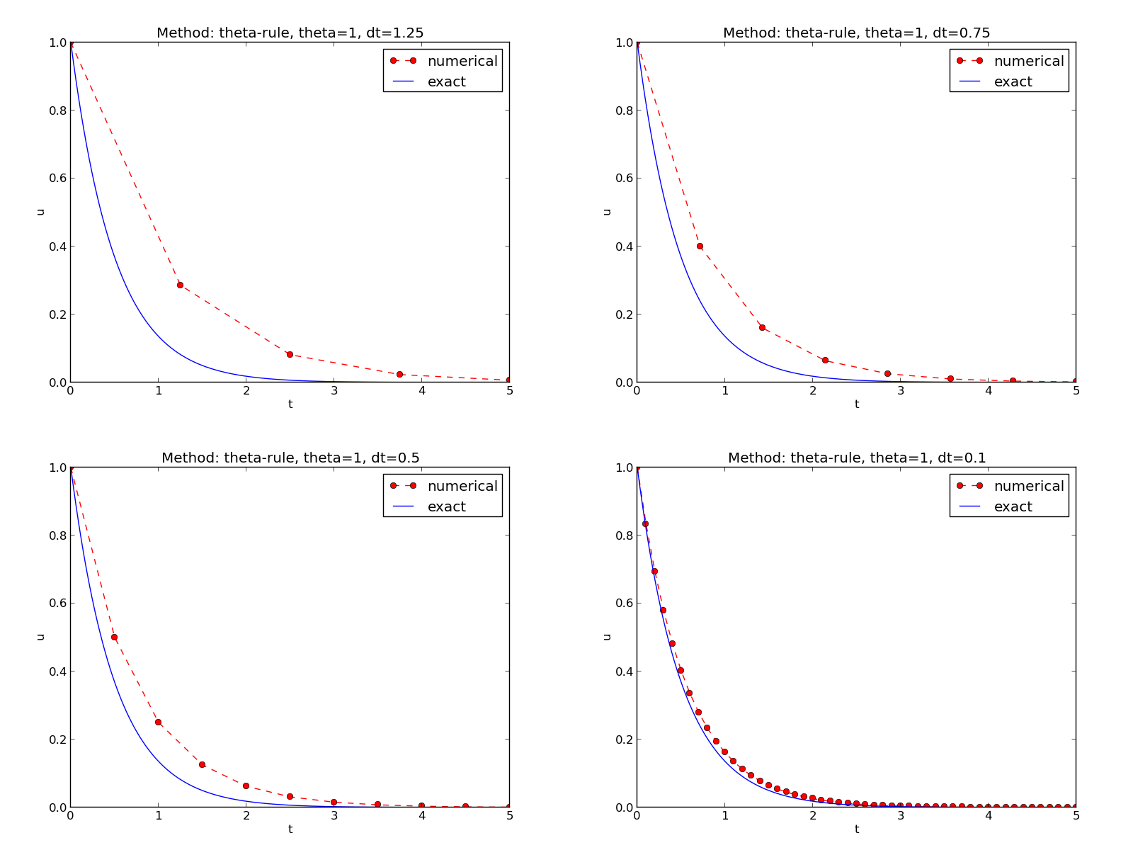
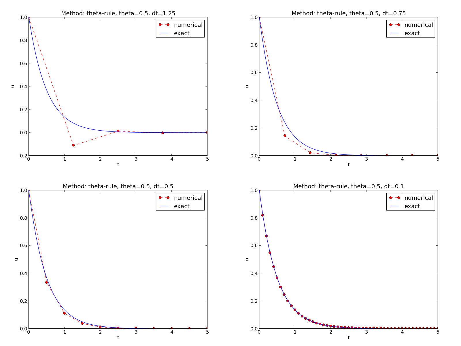
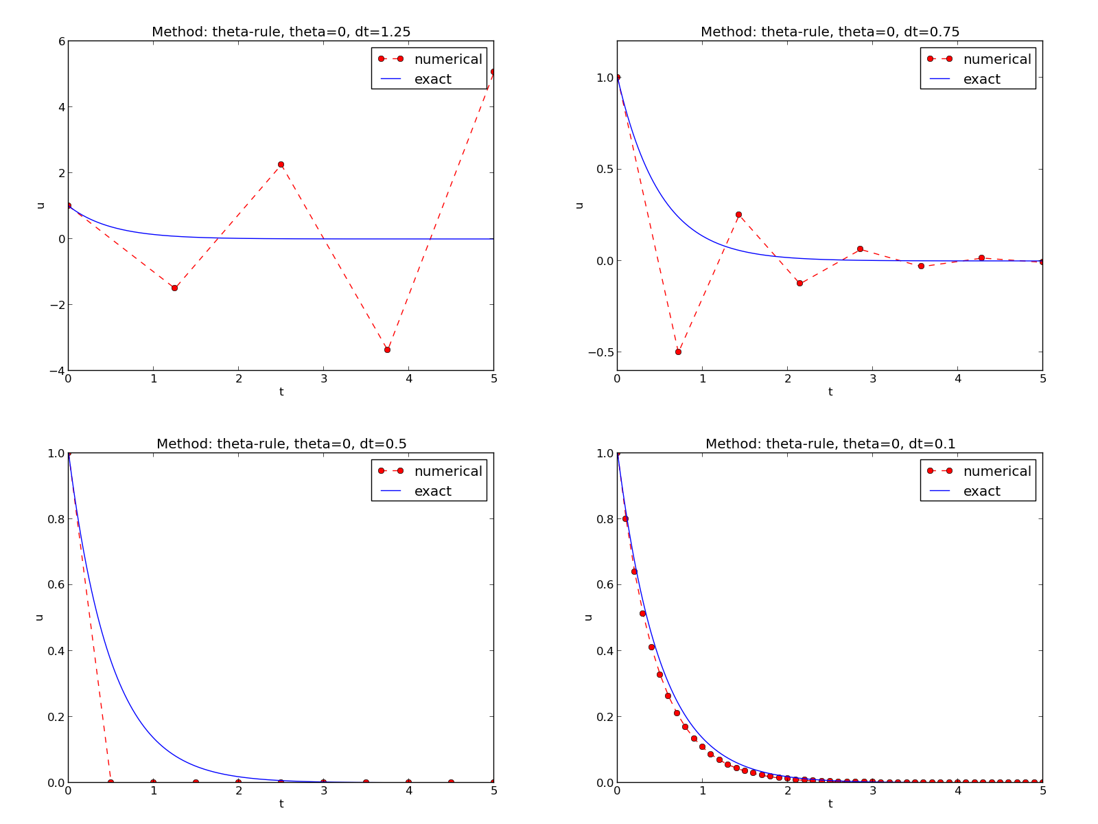
We define a set of numerical experiments where \( I \), \( a \), and \( T \) are fixed, while \( \Delta t \) and \( \theta \) are varied. In particular, \( I=1 \), \( a=2 \), \( \Delta t = 1.25, 0.75, 0.5, 0.1 \).
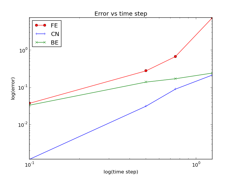
How \( E \) varies with \( \Delta t \) for \( \theta=0,0.5,1 \) is shown in Figure 1.