Finite difference methods for vibration problems

Author:Hans Petter Langtangen Date:Dec 14, 2013

Note: PRELIMINARY VERSION (expect typos)

Vibration problems lead to differential equations with solutions that oscillates in time, typically in a damped or undamped sinusoidal fashion. Such solutions put certain demands on the numerical methods compared to other phenomena whose solutions are monotone. Both the frequency and amplitude of the oscillations need to be accurately handled by the numerical schemes. Most of the reasoning and specific building blocks introduced in the fortcoming text can be reused to construct sound methods for partial differential equations of wave nature in multiple spatial dimensions.

Finite difference discretization

Much of the numerical challenges with computing oscillatory solutions in ODEs and PDEs can be captured by the very simple ODE \(u'' + u =0\) and this is therefore the starting point for method development, implementation, and analysis.

A basic model for vibrations

A system that vibrates without damping and external forcing can be described by ODE problem

(1)\[ u'' + \omega^2u = 0,\quad u(0)=I,\ u'(0)=0,\ t\in (0,T] {\thinspace .}\]

Here, \(\omega\) and \(I\) are given constants. The exact solution of (1) is

(2)\[ u(t) = I\cos (\omega t) {\thinspace .}\]

That is, \(u\) oscillates with constant amplitude \(I\) and angular frequency \(\omega\). The corresponding period of oscillations (i.e., the time between two neighboring peaks in the cosine function) is \(P=2\pi/\omega\). The number of periods per second is \(f=\omega/(2\pi)\) and measured in the unit Hz. Both \(f\) and \(\omega\) are referred to as frequency, but \(\omega\) may be more precisely named angular frequency, measured in rad/s.

In vibrating mechanical systems modeled by (1), \(u(t)\) very often represents a position or a displacement of a particular point in the system. The derivative \(u'(t)\) then has the interpretation of the point’s velocity, and \(u''(t)\) is the associated acceleration. The model (1) is not only applicable to vibrating mechanical systems, but also to oscillations in electrical circuits.

A centered finite difference scheme

To formulate a finite difference method for the model problem (1) we follow the four steps in [Ref1].

Step 1: Discretizing the domain

The domain is discretized by introducing a uniformly partitioned time mesh in the present problem. The points in the mesh are hence \(t_n=n\Delta t\), \(n=0,1,\ldots,N_t\), where \(\Delta t = T/N_t\) is the constant length of the time steps. We introduce a mesh function \(u^n\) for \(n=0,1,\ldots,N_t\), which approximates the exact solution at the mesh points. The mesh function will be computed from algebraic equations derived from the differential equation problem.

Step 2: Fulfilling the equation at discrete time points

The ODE is to be satisfied at each mesh point:

(3)\[ u''(t_n) + \omega^2u(t_n) = 0,\quad n=1,\ldots,N_t {\thinspace .}\]

Step 3: Replacing derivatives by finite differences

The derivative \(u''(t_n)\) is to be replaced by a finite difference approximation. A common second-order accurate approximation to the second-order derivative is

(4)\[ u''(t_n) \approx \frac{u^{n+1}-2u^n + u^{n-1}}{\Delta t^2} {\thinspace .}\]

Inserting (4) in (3) yields

(5)\[ \frac{u^{n+1}-2u^n + u^{n-1}}{\Delta t^2} = -\omega^2 u^n {\thinspace .}\]

We also need to replace the derivative in the initial condition by a finite difference. Here we choose a centered difference, whose accuracy is similar to the centered difference we used for \(u''\):

(6)\[ \frac{u^1-u^{-1}}{2\Delta t} = 0\]\[ {\thinspace .}\]

Step 4: Formulating a recursive algorithm

To formulate the computational algorithm, we assume that we have already computed \(u^{n-1}\) and \(u^n\) such that \(u^{n+1}\) is the unknown value, which we can readily solve for:

(7)\[ u^{n+1} = 2u^n - u^{n-1} - \Delta t^2\omega^2 u^n {\thinspace .}\]

The computational algorithm is simply to apply (7) successively for \(n=1,2,\ldots,N_t-1\). This numerical scheme sometimes goes under the name Stormer’s method or Verlet integration.

Computing the first step

We observe that (7) cannot be used for \(n=0\) since the computation of \(u^1\) then involves the undefined value \(u^{-1}\) at \(t=-\Delta t\). The discretization of the initial condition then come to rescue: (6) implies \(u^{-1} = u^1\) and this relation can be combined with (7) for \(n=1\) to yield a value for \(u^1\):

\[u^1 = 2u^0 - u^{1} - \Delta t^2 \omega^2 u^0,\]

which reduces to

(8)\[ u^1 = u^0 - \frac{1}{2} \Delta t^2 \omega^2 u^0 {\thinspace .}\]

Exercise 5: Use a Taylor polynomial to compute asks you to perform an alternative derivation and also to generalize the initial condition to \(u'(0)=V\neq 0\).

The computational algorithm

The steps for solving (1) becomes

1. \(u^0=I\)
2. compute \(u^1\) from (8)
3. for \(n=1,2,\ldots,N_t-1\):

1. compute \(u^{n+1}\) from (7)

The algorithm is more precisely expressed directly in Python:

t = linspace(0, T, Nt+1)  # mesh points in time
dt = t[1] - t[0]          # constant time step
u = zeros(Nt+1)           # solution

u[0] = I
u[1] = u[0] - 0.5*dt**2*w**2*u[0]
for n in range(1, Nt):
    u[n+1] = 2*u[n] - u[n-1] - dt**2*w**2*u[n]

Remark

In the code, we use w as the symbol for \(\omega\). The reason is that this author prefers w for readability and comparison with the mathematical \(\omega\) instead of the full word omega as variable name.

Operator notation

We may write the scheme using the compact difference notation (see examples in [Ref1]). The difference (4) has the operator notation \([D_tD_t u]^n\) such that we can write:

(9)\[ [D_tD_t u + \omega^2 u = 0]^n {\thinspace .}\]

Note that \([D_tD_t u]^n\) means applying a central difference with step \(\Delta t/2\) twice:

\[[D_t(D_t u)]^n = \frac{[D_t u]^{n+\frac{1}{2}} - [D_t u]^{n-\frac{1}{2}}}{\Delta t}\]

which is written out as

\[\frac{1}{\Delta t}\left(\frac{u^{n+1}-u^n}{\Delta t} - \frac{u^{n}-u^{n-1}}{\Delta t}\right) = \frac{u^{n+1}-2u^n + u^{n-1}}{\Delta t^2} {\thinspace .}\]

The discretization of initial conditions can in the operator notation be expressed as

\[[u = I]^0,\quad [D_{2t} u = 0]^0,\]

where the operator \([D_{2t} u]^n\) is defined as

\[[D_{2t} u]^n = \frac{u^{n+1} - u^{n-1}}{2\Delta t} {\thinspace .}\]

Implementation (1)

Making a solver function

The algorithm from the previous section is readily translated to a complete Python function for computing (returning) \(u^0,u^1,\ldots,u^{N_t}\) and \(t_0,t_1,\ldots,t_{N_t}\), given the input \(I\), \(\omega\), \(\Delta t\), and \(T\):

from numpy import *
from matplotlib.pyplot import *
from vib_empirical_analysis import minmax, periods, amplitudes

def solver(I, w, dt, T):
    """
    Solve u'' + w**2*u = 0 for t in (0,T], u(0)=I and u'(0)=0,
    by a central finite difference method with time step dt.
    """
    dt = float(dt)
    Nt = int(round(T/dt))
    u = zeros(Nt+1)
    t = linspace(0, Nt*dt, Nt+1)

    u[0] = I
    u[1] = u[0] - 0.5*dt**2*w**2*u[0]
    for n in range(1, Nt):
        u[n+1] = 2*u[n] - u[n-1] - dt**2*w**2*u[n]
    return u, t

A function for plotting the numerical and the exact solution is also convenient to have:

def exact_solution(t, I, w):
    return I*cos(w*t)

def visualize(u, t, I, w):
    plot(t, u, 'r--o')
    t_fine = linspace(0, t[-1], 1001)  # very fine mesh for u_e
    u_e = exact_solution(t_fine, I, w)
    hold('on')
    plot(t_fine, u_e, 'b-')
    legend(['numerical', 'exact'], loc='upper left')
    xlabel('t')
    ylabel('u')
    dt = t[1] - t[0]
    title('dt=%g' % dt)
    umin = 1.2*u.min();  umax = -umin
    axis([t[0], t[-1], umin, umax])
    savefig('vib1.png')
    savefig('vib1.pdf')
    savefig('vib1.eps')

A corresponding main program calling these functions for a simulation of a given number of periods (num_periods) may take the form

I = 1
w = 2*pi
dt = 0.05
num_periods = 5
P = 2*pi/w    #  one period
T = P*num_periods
u, t = solver(I, w, dt, T)
visualize(u, t, I, w, dt)

Adjusting some of the input parameters on the command line can be handy. Here is a code segment using the ArgumentParser tool in the argparse module to define option value (--option value) pairs on the command line:

import argparse
parser = argparse.ArgumentParser()
parser.add_argument('--I', type=float, default=1.0)
parser.add_argument('--w', type=float, default=2*pi)
parser.add_argument('--dt', type=float, default=0.05)
parser.add_argument('--num_periods', type=int, default=5)
a = parser.parse_args()
I, w, dt, num_periods = a.I, a.w, a.dt, a.num_periods

A typical execution goes like

Terminal> python vib_undamped.py --num_periods 20 --dt 0.1

Computing \(u'\)

In mechanical vibration applications one is often interested in computing the velocity \(v(t)=u'(t)\) after \(u(t)\) has been computed. This can be done by a central difference,

\[v(t_n)=u'(t_n) \approx v^n = \frac{u^{n+1}-u^{n-1}}{2\Delta t} = [D_{2t}u]^n {\thinspace .}\]

This formula applies for all inner mesh points, \(n=1,\ldots,N_t-1\). For \(n=0\) we have that \(v(0)\) is given by the initial condition on \(u'(0)\), and for \(n=N_t\) we can use a one-sided, backward difference: \(v^n=[D_t^-u]^n\).

Appropriate vectorized Python code becomes

v = np.zeros_like(u)
v[1:-1] = (u[2:] - u[:-2])/(2*dt)  # internal mesh points
v[0] = V                           # Given boundary condition u'(0)
v[-1] = (u[-1] - u[-2])/dt         # backward difference

Verification (1)

Manual calculation

The simplest type of verification, which is also instructive for understanding the algorithm, is to compute \(u^1\), \(u^2\), and \(u^3\) with the aid of a calculator and make a function for comparing these results with those from the solver function. We refer to the test_three_steps function in the file vib_undamped.py for details.

Testing very simple solutions

Constructing test problems where the exact solution is constant or linear helps initial debugging and verification as one expects any reasonable numerical method to reproduce such solutions to machine precision. Second-order accurate methods will often also reproduce a quadratic solution. Here \([D_tD_tt^2]^n=2\), which is the exact result. A solution \(u=t^2\) leads to \(u''+\omega^2 u=2 + (\omega t)^2\neq 0\). We must therefore add a source in the equation: \(u'' + \omega^2 u = f\) to allow a solution \(u=t^2\) for \(f=(\omega t)^2\). By simple insertion we can show that the mesh function \(u^n = t_n^2\) is also a solution of the discrete equations. Problem 1: Use linear/quadratic functions for verification asks you to carry out all details with showing that linear and quadratic solutions are solutions of the discrete equations. Such results are very useful for debugging and verification.

Checking convergence rates

Empirical computation of convergence rates, as explained for a simple ODE model, yields a good method for verification. The function below

• performs \(m\) simulations with halved time steps: \(2^{-i}\Delta t\), \(i=0,\ldots,m-1\),
• computes the \(L^2\) norm of the error, \(E=\sqrt{2^{-i}\Delta t\sum_{n=0}^{N_t-1}(u^n-{u_{\small\mbox{e}}}(t_n))^2}\) in each case,
• estimates the convergence rates \(r_i\) based on two consecutive experiments \((\Delta t_{i-1}, E_{i-1})\) and \((\Delta t_{i}, E_{i})\), assuming \(E_i=C\Delta t_i^{r_i}\) and \(E_{i-1}=C\Delta t_{i-1}^{r_i}\). From these equations it follows that \(r_{i-1} = \ln (E_{i-1}/E_i)/\ln (\Delta t_{i-1}/\Delta t_i)\), for \(i=1,\ldots,m-1\).

All the implementational details appear below.

def convergence_rates(m, num_periods=8):
    """
    Return m-1 empirical estimates of the convergence rate
    based on m simulations, where the time step is halved
    for each simulation.
    """
    w = 0.35; I = 0.3
    dt = 2*pi/w/30  # 30 time step per period 2*pi/w
    T = 2*pi/w*num_periods
    dt_values = []
    E_values = []
    for i in range(m):
        u, t = solver(I, w, dt, T)
        u_e = exact_solution(t, I, w)
        E = sqrt(dt*sum((u_e-u)**2))
        dt_values.append(dt)
        E_values.append(E)
        dt = dt/2

    r = [log(E_values[i-1]/E_values[i])/
         log(dt_values[i-1]/dt_values[i])
         for i in range(1, m, 1)]
    return r

The returned r list has its values equal to 2.00, which is in excellent agreement with what is expected from the second-order finite difference approximation \([D_tD_tu]^n\) and other theoretical measures of the error in the numerical method. The final r[-1] value is a good candidate for a unit test:

def test_convergence_rates():
    r = convergence_rates(m=5, num_periods=8)
    # Accept rate to 1 decimal place
    nt.assert_almost_equal(r[-1], 2.0, places=1)

The complete code appears in the file vib_undamped.py.

Long time simulations

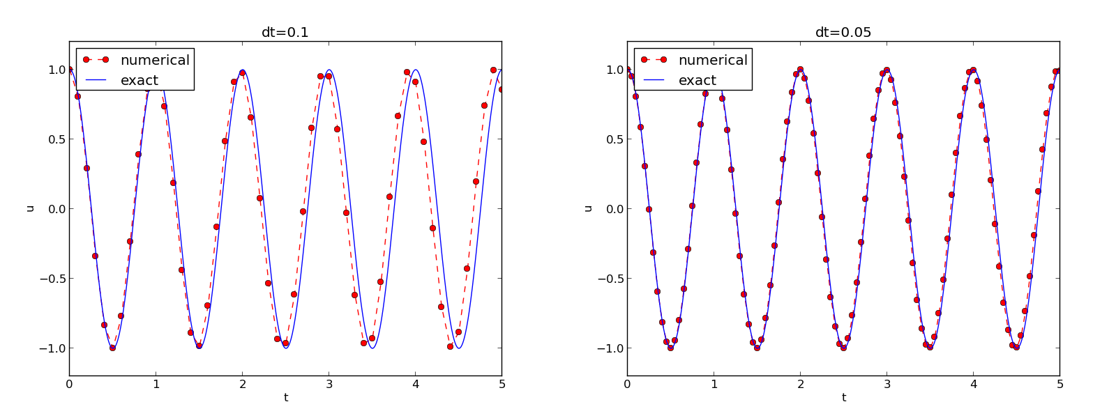
Figure Effect of halving the time step shows a comparison of the exact and numerical solution for \(\Delta t=0.1, 0.05\) and \(w=2\pi\). From the plot we make the following observations:

• The numerical solution seems to have correct amplitude.
• There is a phase error which is reduced by reducing the time step.
• The total phase error grows with time.

By phase error we mean that the peaks of the numerical solution have incorrect positions compared with the peaks of the exact cosine solution. This effect can be understood as if also the numerical solution is on the form \(I\cos\tilde\omega t\), but where \(\tilde\omega\) is not exactly equal to \(\omega\). Later, we shall mathematically quantify this numerical frequency \(\tilde\omega\).

Effect of halving the time step

Using a moving plot window

In vibration problems it is often of interest to investigate the system’s behavior over long time intervals. Errors in the phase may then show up as crucial. Let us investigate long time series by introducing a moving plot window that can move along with the \(p\) most recently computed periods of the solution. The SciTools package contains a convenient tool for this: MovingPlotWindow. Typing pydoc scitools.MovingPlotWindow shows a demo and description of usage. The function below illustrates the usage and is invoked in the vib_undamped.py code if the number of periods in the simulation exceeds 10:

def visualize_front(u, t, I, w, savefig=False):
    """
    Visualize u and the exact solution vs t, using a
    moving plot window and continuous drawing of the
    curves as they evolve in time.
    Makes it easy to plot very long time series.
    """
    import scitools.std as st
    from scitools.MovingPlotWindow import MovingPlotWindow

    P = 2*pi/w  # one period
    umin = 1.2*u.min();  umax = -umin
    plot_manager = MovingPlotWindow(
        window_width=8*P,
        dt=t[1]-t[0],
        yaxis=[umin, umax],
        mode='continuous drawing')
    for n in range(1,len(u)):
        if plot_manager.plot(n):
            s = plot_manager.first_index_in_plot
            st.plot(t[s:n+1], u[s:n+1], 'r-1',
                    t[s:n+1], I*cos(w*t)[s:n+1], 'b-1',
                    title='t=%6.3f' % t[n],
                    axis=plot_manager.axis(),
                    show=not savefig) # drop window if savefig
            if savefig:
                filename = 'tmp_vib%04d.png' % n
                st.savefig(filename)
                print 'making plot file', filename, 'at t=%g' % t[n]
        plot_manager.update(n)

Running

Terminal> python vib_undamped.py --dt 0.05 --num_periods 40

makes the simulation last for 40 periods of the cosine function. With the moving plot window we can follow the numerical and exact solution as time progresses, and we see from this demo that the phase error is small in the beginning, but then becomes more prominent with time. Running vib_undamped.py with \(\Delta t=0.1\) clearly shows that the phase errors become significant even earlier in the time series and destroys the solution.

Making a movie file

The visualize_front function stores all the plots in files whose names are numbered: tmp_vib0000.png, tmp_vib0001.png, tmp_vib0002.png, and so on. From these files we may make a movie. The Flash format is popular,

Terminal> avconv -r 12 -i tmp_vib%04d.png -vcodec flv movie.flv

The avconv program can be replaced by the ffmpeg program in the above command if desired. The -r option should come first and describes the number of frames per second in the movie. The -i option describes the name of the plot files. Other formats can be generated by changing the video codec and equipping the movie file with the right extension:

Format	Codec and filename
Flash	-vcodec flv movie.flv
MP4	-vcodec libx64 movie.mp4
Webm	-vcodec libvpx movie.webm
Ogg	-vcodec libtheora movie.ogg

The movie file can be played by some video player like vlc, mplayer, gxine, or totem, e.g.,

Terminal> vlc movie.webm

A web page can also be used to play the movie. Today’s standard is to use the HTML5 video tag:

<video autoplay loop controls
       width='640' height='365' preload='none'>
<source src='movie.webm'  type='video/webm; codecs="vp8, vorbis"'>
</video>

Caution: number the plot files correctly

To ensure that the individual plot frames are shown in correct order, it is important to number the files with zero-padded numbers (0000, 0001, 0002, etc.). The printf format %04d specifies an integer in a field of width 4, padded with zeros from the left. A simple Unix wildcard file specification like tmp_vib*.png will then list the frames in the right order. If the numbers in the filenames were not zero-padded, the frame tmp_vib11.png would appear before tmp_vib2.png in the movie.

Using a line-by-line ascii plotter

Plotting functions vertically, line by line, in the terminal window using ascii characters only is a simple, fast, and convenient visualization technique for long time series (the time arrow points downward). The tool scitools.avplotter.Plotter makes it easy to create such plots:

def visualize_front_ascii(u, t, I, w, fps=10):
    """
    Plot u and the exact solution vs t line by line in a
    terminal window (only using ascii characters).
    Makes it easy to plot very long time series.
    """
    from scitools.avplotter import Plotter
    import time
    P = 2*pi/w
    umin = 1.2*u.min();  umax = -umin

    p = Plotter(ymin=umin, ymax=umax, width=60, symbols='+o')
    for n in range(len(u)):
        print p.plot(t[n], u[n], I*cos(w*t[n])), \
              '%.1f' % (t[n]/P)
        time.sleep(1/float(fps))

if __name__ == '__main__':
    main()

The call p.plot returns a line of text, with the \(t\) axis marked and a symbol + for the first function (u) and o for the second function (the exact solution). Here we append this text a time counter reflecting how many periods the current time point corresponds to. A typical output (\(\omega =2\pi\), \(\Delta t=0.05\)) looks like this:

                         |                       o+      14.0
                         |                      + o      14.0
                         |                  +    o       14.1
                         |             +     o           14.1
                         |     +        o                14.2
                        +|       o                       14.2
                +        |                               14.2
         +       o       |                               14.3
    +     o              |                               14.4
 +   o                   |                               14.4
+o                       |                               14.5
o +                      |                               14.5
 o    +                  |                               14.6
     o      +            |                               14.6
          o        +     |                               14.7
                 o       | +                             14.7
                         |        +                      14.8
                         |       o       +               14.8
                         |              o     +          14.9
                         |                   o   +       14.9
                         |                       o+      15.0

Empirical analysis of the solution

For oscillating functions like those in Figure Effect of halving the time step we may compute the amplitude and frequency (or period) empirically. That is, we run through the discrete solution points \((t_n, u_n)\) and find all maxima and minima points. The distance between two consecutive maxima (or minima) points can be used as estimate of the local period, while half the difference between the \(u\) value at a maximum and a nearby minimum gives an estimate of the local amplitude.

The local maxima are the points where

\[\begin{split}u^{n-1} < u^n > u^{n+1},\quad n=1,\ldots,N_t-1,\end{split}\]

and the local minima are recognized by

\[\begin{split}u^{n-1} > u^n < u^{n+1},\quad n=1,\ldots,N_t-1 {\thinspace .}\end{split}\]

In computer code this becomes

def minmax(t, u):
    minima = []; maxima = []
    for n in range(1, len(u)-1, 1):
        if u[n-1] > u[n] < u[n+1]:
            minima.append((t[n], u[n]))
        if u[n-1] < u[n] > u[n+1]:
            maxima.append((t[n], u[n]))
    return minima, maxima

Note that the returned objects are list of tuples.

Let \((t_i, e_i)\), \(i=0,\ldots,M-1\), be the sequence of all the \(M\) maxima points, where \(t_i\) is the time value and \(e_i\) the corresponding \(u\) value. The local period can be defined as \(p_i=t_{i+1}-t_i\). With Python syntax this reads

def periods(maxima):
    p = [extrema[n][0] - maxima[n-1][0]
         for n in range(1, len(maxima))]
    return np.array(p)

The list p created by a list comprehension is converted to an array since we probably want to compute with it, e.g., find the corresponding frequencies 2*pi/p.

Having the minima and the maxima, the local amplitude can be calculated as the difference between two neighboring minimum and maximum points:

def amplitudes(minima, maxima):
    a = [(abs(maxima[n][1] - minima[n][1]))/2.0
         for n in range(min(len(minima),len(maxima)))]
    return np.array(a)

The code segments are found in the file vib_empirical_analysis.py.

Visualization of the periods p or the amplitudes a it is most conveniently done with just a counter on the horizontal axis, since a[i] and p[i] correspond to the \(i\)-th amplitude estimate and the \(i\)-th period estimate, respectively. There is no unique time point associated with either of these estimate since values at two different time points were used in the computations.

In the analysis of very long time series, it is advantageous to compute and plot p and a instead of \(u\) to get an impression of the development of the oscillations.

Analysis of the numerical scheme

Deriving an exact numerical solution

After having seen the phase error grow with time in the previous section, we shall now quantify this error through mathematical analysis. The key tool in the analysis will be to establish an exact solution of the discrete equations. The difference equation (7) has constant coefficients and is homogeneous. The solution is then \(u^n=CA^n\), where \(A\) is some number to be determined from the differential equation and \(C\) is determined from the initial condition (\(C=I\)). Recall that \(n\) in \(u^n\) is a superscript labeling the time level, while \(n\) in \(A^n\) is an exponent. With oscillating functions as solutions, the algebra will be considerably simplified if we seek an \(A\) on the form

\[A=e^{i\tilde\omega \Delta t},\]

and solve for the numerical frequency \(\tilde\omega\) rather than \(A\). Note that \(i=\sqrt{-1}\) is the imaginary unit. (Using a complex exponential function gives simpler arithmetics than working with a sine or cosine function.) We have

\[A^n = e^{i\tilde\omega \Delta t\, n}=e^{i\tilde\omega t} = \cos (\tilde\omega t) + i\sin(\tilde \omega t) {\thinspace .}\]

The physically relevant numerical solution can be taken as the real part of this complex expression.

The calculations goes as

\[\begin{split}[D_tD_t u]^n &= \frac{u^{n+1} - 2u^n + u^{n-1}}{\Delta t^2}\\ &= I\frac{A^{n+1} - 2A^n + A^{n-1}}{\Delta t^2}\\ &= I\frac{\exp{(i\tilde\omega(t+\Delta t))} - 2\exp{(i\tilde\omega t)} + \exp{(i\tilde\omega(t-\Delta t))}}{\Delta t^2}\\ &= I\exp{(i\tilde\omega t)}\frac{1}{\Delta t^2}\left(\exp{(i\tilde\omega(\Delta t))} + \exp{(i\tilde\omega(-\Delta t))} - 2\right)\\ &= I\exp{(i\tilde\omega t)}\frac{2}{\Delta t^2}\left(\cosh(i\tilde\omega\Delta t) -1 \right)\\ &= I\exp{(i\tilde\omega t)}\frac{2}{\Delta t^2}\left(\cos(\tilde\omega\Delta t) -1 \right)\\ &= -I\exp{(i\tilde\omega t)}\frac{4}{\Delta t^2}\sin^2(\frac{\tilde\omega\Delta t}{2})\end{split}\]

The last line follows from the relation \(\cos x - 1 = -2\sin^2(x/2)\) (try cos(x)-1 in wolframalpha.com to see the formula).

The scheme (7) with \(u^n=Ie^{i\omega\tilde\Delta t\, n}\) inserted now gives

\[-Ie^{i\tilde\omega t}\frac{4}{\Delta t^2}\sin^2(\frac{\tilde\omega\Delta t}{2}) + \omega^2 Ie^{i\tilde\omega t} = 0,\]

which after dividing by \(Ie^{i\tilde\omega t}\) results in

\[\frac{4}{\Delta t^2}\sin^2(\frac{\tilde\omega\Delta t}{2}) = \omega^2 {\thinspace .}\]

The first step in solving for the unknown \(\tilde\omega\) is

\[\sin^2(\frac{\tilde\omega\Delta t}{2}) = \left(\frac{\omega\Delta t}{2}\right)^2 {\thinspace .}\]

Then, taking the square root, applying the inverse sine function, and multiplying by \(2/\Delta t\), results in

(10)\[ \tilde\omega = \pm \frac{2}{\Delta t}\sin^{-1}\left(\frac{\omega\Delta t}{2}\right) {\thinspace .}\]

The first observation of (10) tells that there is a phase error since the numerical frequency \(\tilde\omega\) never equals the exact frequency \(\omega\). But how good is the approximation (10)? That is, what is the error \(\omega - \tilde\omega\) or \(\tilde\omega/\omega\)? Taylor series expansion for small \(\Delta t\) may give an expression that is easier to understand than the complicated function in (10):

>>> from sympy import *
>>> dt, w = symbols('dt w')
>>> w_tilde_e = 2/dt*asin(w*dt/2)
>>> w_tilde_series = w_tilde_e.series(dt, 0, 4)
>>> print w_tilde_series
w + dt**2*w**3/24 + O(dt**4)

This means that

(11)\[ \tilde\omega = \omega\left( 1 + \frac{1}{24}\omega^2\Delta t^2\right) + {\mathcal{O}(\Delta t^4)} {\thinspace .}\]

The error in the numerical frequency is of second-order in \(\Delta t\), and the error vanishes as \(\Delta t\rightarrow 0\). We see that \(\tilde\omega > \omega\) since the term \(\omega^3\Delta t^2/24 >0\) and this is by far the biggest term in the series expansion for small \(\omega\Delta t\). A numerical frequency that is too large gives an oscillating curve that oscillates too fast and therefore “lags behind” the exact oscillations, a feature that can be seen in the plots.

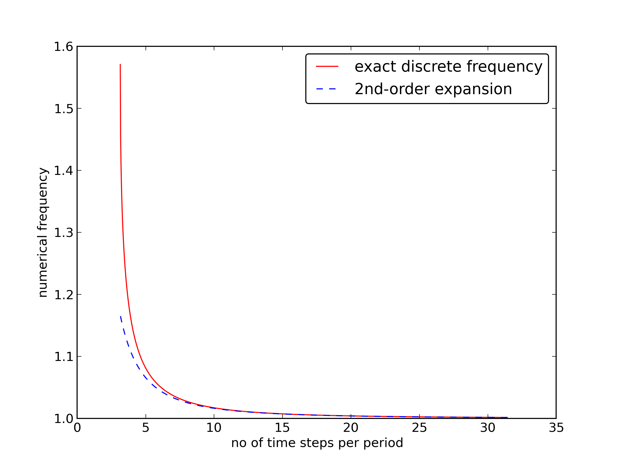
Figure Exact discrete frequency and its second-order series expansion plots the discrete frequency (10) and its approximation (11) for \(\omega =1\) (based on the program vib_plot_freq.py). Although \(\tilde\omega\) is a function of \(\Delta t\) in (11), it is misleading to think of \(\Delta t\) as the important discretization parameter. It is the product \(\omega\Delta t\) that is the key discretization parameter. This quantity reflects the number of time steps per period of the oscillations. To see this, we set \(P=N_P\Delta t\), where \(P\) is the length of a period, and \(N_P\) is the number of time steps during a period. Since \(P\) and \(\omega\) are related by \(P=2\pi/\omega\), we get that \(\omega\Delta t = 2\pi/N_P\), which shows that \(\omega\Delta t\) is directly related to \(N_P\).

The plot shows that at least \(N_P\sim 25-30\) points per period are necessary for reasonable accuracy, but this depends on the length of the simulation (\(T\)) as the total phase error due to the frequency error grows linearly with time (see Exercise 2: Show linear growth of the phase with time).

Exact discrete frequency and its second-order series expansion

Exact discrete solution

Perhaps more important than the \(\tilde\omega = \omega + {\cal O}(\Delta t^2)\) result found above is the fact that we have an exact discrete solution of the problem:

(12)\[ u^n = I\cos\left(\tilde\omega n\Delta t\right),\quad \tilde\omega = \frac{2}{\Delta t}\sin^{-1}\left(\frac{\omega\Delta t}{2}\right) {\thinspace .}\]

We can then compute the error mesh function

(13)\[ e^n = {u_{\small\mbox{e}}}(t_n) - u^n = I\cos\left(\omega n\Delta t\right) - I\cos\left(\tilde\omega n\Delta t\right) {\thinspace .}\]

In particular, we can use this expression to show convergence of the numerical scheme, i.e., \(e^n\rightarrow 0\) as \(\Delta t\rightarrow 0\). We have that

\[\lim_{\Delta t\rightarrow 0} \tilde\omega = \lim_{\Delta t\rightarrow 0} \frac{2}{\Delta t}\sin^{-1}\left(\frac{\omega\Delta t}{2}\right) = \omega,\]

by L’Hopital’s rule or simply asking (2/x)*asin(w*x/2) as x->0 in WolframAlpha. Therefore, \(\tilde\omega\rightarrow\omega\), and the two terms in \(e^n\) cancel each other in the limit \(\Delta t\rightarrow 0\).

The error mesh function is ideal for verification purposes (and you are encouraged to make a test based on (12) in Exercise 10: Use an exact discrete solution for verification).

The global error

To achieve more analytical insight into the nature of the global error, we can Taylor expand the error mesh function. Since \(\tilde\omega\) contains \(\Delta t\) in the denominator we use the series expansion for \(\tilde\omega\) inside the cosine function:

>>> dt, w, t = symbols('dt w t')
>>> w_tilde_e = 2/dt*asin(w*dt/2)
>>> w_tilde_series = w_tilde_e.series(dt, 0, 4)
>>> # Get rid of O() term
>>> w_tilde_series = sum(w_tilde_series.as_ordered_terms()[:-1])
>>> w_tilde_series
dt**2*w**3/24 + w
>>> error = cos(w*t) - cos(w_tilde_series*t)
>>> error.series(dt, 0, 6)
dt**2*t*w**3*sin(t*w)/24 + dt**4*t**2*w**6*cos(t*w)/1152 + O(dt**6)
>>> error.series(dt, 0, 6).as_leading_term(dt)
dt**2*t*w**3*sin(t*w)/24

This means that the leading order global (true) error at a point \(t\) is proportional to \(\omega^3t\Delta t^2\). Setting \(t=n\Delta t\) and replacing \(\sin(\omega t)\) by its maximum value 1, we have the analytical leading-order expression

\[e^n = \frac{1}{24}n\omega^3\Delta t^3,\]

and the \(\ell^2\) norm of this error can be computed as

\[||e^n||_{\ell^2}^2 = \Delta t\sum_{n=0}^{N_t} \frac{1}{24^2}n^2\omega^6\Delta t^6 =\frac{1}{24^2}\omega^6\Delta t^7 \sum_{n=0}^{N_t} n^2{\thinspace .}\]

The sum \(\sum_{n=0}^{N_t} n^2\) is approximately equal to \(\frac{1}{3}N_t^3\). Replacing \(N_t\) by \(T/\Delta t\) and taking the square root gives the expression

\[||e^n||_{\ell^2} = \frac{1}{24}\sqrt{\frac{T^3}{3}}\omega^3\Delta t^2,\]

which shows that also the integrated error is proportional to \(\Delta t^2\).

Stability

Looking at (12), it appears that the numerical solution has constant and correct amplitude, but an error in the frequency (phase error). However, there is another error that is more serious, namely an unstable growing amplitude that can occur of \(\Delta t\) is too large.

We realize that a constant amplitude demands \(\tilde\omega\) to be a real number. A complex \(\tilde\omega\) is indeed possible if the argument \(x\) of \(\sin^{-1}(x)\) has magnitude larger than unity: \(|x|>1\) (type asin(x) in wolframalpha.com to see basic properties of \(\sin^{-1} (x)\)). A complex \(\tilde\omega\) can be written \(\tilde\omega = \tilde\omega_r + i\tilde\omega_i\). Since \(\sin^{-1}(x)\) has a negative imaginary part for \(x>1\), \(\tilde\omega_i < 0\), it means that \(\exp{(i\omega\tilde t)}=\exp{(-\tilde\omega_i t)}\exp{(i\tilde\omega_r t)}\) will lead to exponential growth in time because \(\exp{(-\tilde\omega_i t)}\) with \(\tilde\omega_i <0\) has a positive exponent.

We do not tolerate growth in the amplitude and we therefore have a stability criterion arising from requiring the argument \(\omega\Delta t/2\) in the inverse sine function to be less than one:

\[\frac{\omega\Delta t}{2} \leq 1\quad\Rightarrow\quad \Delta t \leq \frac{2}{\omega} {\thinspace .}\]

With \(\omega =2\pi\), \(\Delta t > \pi^{-1} = 0.3183098861837907\) will give growing solutions. Figure Growing, unstable solution because of a time step slightly beyond the stability limit displays what happens when \(\Delta t =0.3184\), which is slightly above the critical value: \(\Delta t =\pi^{-1} + 9.01\cdot 10^{-5}\).

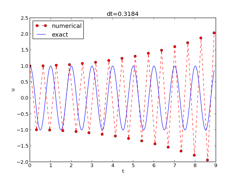
Growing, unstable solution because of a time step slightly beyond the stability limit

About the accuracy at the stability limit

An interesting question is whether the stability condition \(\Delta t < 2/\omega\) is unfortunate, or more precisely: would it be meaningful to take larger time steps to speed up computations? The answer is a clear no. At the stability limit, we have that \(\sin^{-1}\omega\Delta t/2 = \sin^{-1} 1 = \pi/2\), and therefore \(\tilde\omega = \pi/\Delta t\). (Note that the approximate formula (11) is very inaccurate for this value of \(\Delta t\) as it predicts \(\tilde\omega = 2.34/pi\), which is a 25 percent reduction.) The corresponding period of the numerical solution is \(\tilde P=2\pi/\tilde\omega = 2\Delta t\), which means that there is just one time step \(\Delta t\) between a peak and a through in the numerical solution. This is the shortest possible wave that can be represented in the mesh. In other words, it is not meaningful to use a larger time step than the stability limit.

Also, the phase error when \(\Delta t = 2/\omega\) is severe: Figure Numerical solution with :math:`Delta t` exactly at the stability limit shows a comparison of the numerical and analytical solution with \(\omega = 2\pi\) and \(\Delta t = 2/\omega = \pi^{-1}\). Already after one period, the numerical solution has a through while the exact solution has a peak (!). The error in frequency when \(\Delta t\) is at the stability limit becomes \(\omega - \tilde\omega = \omega(1-\pi/2)\approx -0.57\omega\). The corresponding error in the period is \(P - \tilde P \approx 0.36P\). The error after \(m\) periods is then \(0.36mP\). This error has reach half a period when \(m=1/(2\cdot 0.36)\approx 1.38\), which theoretically confirms the observations in Figure Numerical solution with :math:`Delta t` exactly at the stability limit that the numerical solution is a through ahead of a peak already after one and a half period.

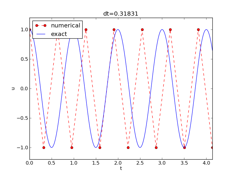
Numerical solution with :math:`Delta t` exactly at the stability limit

Summary

From the accuracy and stability analysis we can draw three important conclusions:

1. The key parameter in the formulas is \(p=\omega\Delta t\). The period of oscillations is \(P=2\pi/\omega\), and the number of time steps per period is \(N_P=P/\Delta t\). Therefore, \(p=\omega\Delta t = 2\pi N_P\), showing that the critical parameter is the number of time steps per period. The smallest possible \(N_P\) is 2, showing that \(p\in (0,\pi]\).
2. Provided \(p\leq 2\), the amplitude of the numerical solution is constant.
3. The numerical solution exhibits a relative phase error \(\tilde\omega/\omega \approx 1 + \frac{1}{24}p^2\). This error leads to wrongly displaced peaks of the numerical solution, and the error in peak location grows linearly with time (see Exercise 2: Show linear growth of the phase with time).

Alternative schemes based on 1st-order equations

A standard technique for solving second-order ODEs is to rewrite them as a system of first-order ODEs and then apply the vast collection of methods for first-order ODE systems. Given the second-order ODE problem

\[u'' + \omega^2 u = 0,\quad u(0)=I,\ u'(0)=0,\]

we introduce the auxiliary variable \(v=u'\) and express the ODE problem in terms of first-order derivatives of \(u\) and \(v\):

(14)\[ u' = v,\]

(15)\[ v' = -\omega^2 u\]\[ {\thinspace .}\]

The initial conditions become \(u(0)=I\) and \(v(0)=0\).

Standard methods for 1st-order ODE systems

The Forward Euler scheme

A Forward Euler approximation to our \(2\times 2\) system of ODEs (14)-(15) becomes

\[\lbrack D_t^+ u = v\rbrack^n, \lbrack D_t^+ v = -\omega^2 u\rbrack^n,\]

or written out,

(16)\[ u^{n+1} = u^n + \Delta t v^n,\]

(17)\[ v^{n+1} = v^n -\Delta t \omega^2 u^n\]\[ {\thinspace .}\]

Let us briefly compare this Forward Euler method with the centered difference scheme for the second-order differential equation. We have from (16) and (17) applied at levels \(n\) and \(n-1\) that

\[u^{n+1} = u^n + \Delta t v^n = u^n + \Delta t (v^{n-1} -\Delta t \omega^2 u^{n-1}{\thinspace .}\]

Since from (16)

\[v^{n-1} = \frac{1}{\Delta t}(u^{n}-u^{n-1}),\]

it follows that

\[u^{n+1} = 2u^n - u^{n-1} -\Delta t^2\omega^2 u^{n-1},\]

which is very close to the centered difference scheme, but the last term is evaluated at \(t_{n-1}\) instead of \(t_n\). This difference is actually crucial for the accuracy of the Forward Euler method applied to vibration problems.

The Backward Euler scheme

A Backward Euler approximation the ODE system is equally easy to write up in the operator notation:

\[\lbrack D_t^- u = v\rbrack^{n+1},\]

\[\lbrack D_t^- v = -\omega u\rbrack^{n+1} {\thinspace .}\]

This becomes a coupled system for \(u^{n+1}\) and \(v^{n+1}\):

\[u^{n+1} - \Delta t v^{n+1} = u^{n},\]

\[v^{n+1} + \Delta t \omega^2 u^{n+1} = v^{n} {\thinspace .}\]

The Crank-Nicolson scheme

The Crank-Nicolson scheme takes this form in the operator notation:

\[\lbrack D_t u = \overline{v}^t\rbrack^{n+\frac{1}{2}},\]

\[\lbrack D_t v = -\omega \overline{u}^t\rbrack^{n+\frac{1}{2}} {\thinspace .}\]

Writing the equations out shows that is also a coupled system:

\[u^{n+1} - \frac{1}{2}\Delta t v^{n+1} = u^{n} + \frac{1}{2}\Delta t v^{n},\]

\[v^{n+1} + \frac{1}{2}\Delta t \omega^2 u^{n+1} = v^{n} - \frac{1}{2}\Delta t \omega^2 u^{n} {\thinspace .}\]

Comparison of schemes

We can easily compare methods like the ones above (and many more!) with the aid of the Odespy package. Below is a sketch of the code.

import odespy
import numpy as np

def f(u, t, w=1):
    u, v = u  # u is array of length 2 holding our [u, v]
    return [v, -w**2*u]

def run_solvers_and_plot(solvers, timesteps_per_period=20,
                         num_periods=1, I=1, w=2*np.pi):
    P = 2*np.pi/w  # duration of one period
    dt = P/timesteps_per_period
    Nt = num_periods*timesteps_per_period
    T = Nt*dt
    t_mesh = np.linspace(0, T, Nt+1)

    legends = []
    for solver in solvers:
        solver.set(f_kwargs={'w': w})
        solver.set_initial_condition([I, 0])
        u, t = solver.solve(t_mesh)

There is quite some more code dealing with plots also, and we refer to the source file vib_undamped_odespy.py for details. Observe that keyword arguments in f(u,t,w=1) can be supplied through a solver parameter f_kwargs (dictionary).

Specification of the Forward Euler, Backward Euler, and Crank-Nicolson schemes is done like this:

solvers = [
    odespy.ForwardEuler(f),
    # Implicit methods must use Newton solver to converge
    odespy.BackwardEuler(f, nonlinear_solver='Newton'),
    odespy.CrankNicolson(f, nonlinear_solver='Newton'),
    ]

The vib_undamped_odespy.py program makes two plots of the computed solutions with the various methods in the solvers list: one plot with \(u(t)\) versus \(t\), and one phase plane plot where \(v\) is plotted against \(u\). That is, the phase plane plot is the curve \((u(t),v(t))\) parameterized by \(t\). Analytically, \(u=I\cos(\omega t)\) and \(v=u'=-\omega I\sin(\omega t)\). The exact curve \((u(t),v(t))\) is therefore an ellipse, which often looks like a circle in a plot if the axes are automatically scaled. The important feature, however, is that exact curve \((u(t),v(t))\) is closed and repeats itself for every period. Not all numerical schemes are capable to do that, meaning that the amplitude instead shrinks or grows with time.

The Forward Euler scheme in Figure Comparison of classical schemes in the phase plane has a pronounced spiral curve, pointing to the fact that the amplitude steadily grows, which is also evident in Figure Comparison of classical schemes. The Backward Euler scheme has a similar feature, except that the spriral goes inward and the amplitude is significantly damped. The changing amplitude and the sprial form decreases with decreasing time step. The Crank-Nicolson scheme looks much more accurate. In fact, these plots tell that the Forward and Backward Euler schemes are not suitable for solving our ODEs with oscillating solutions.

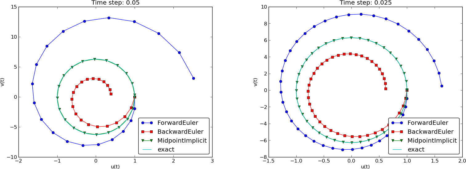
Comparison of classical schemes in the phase plane

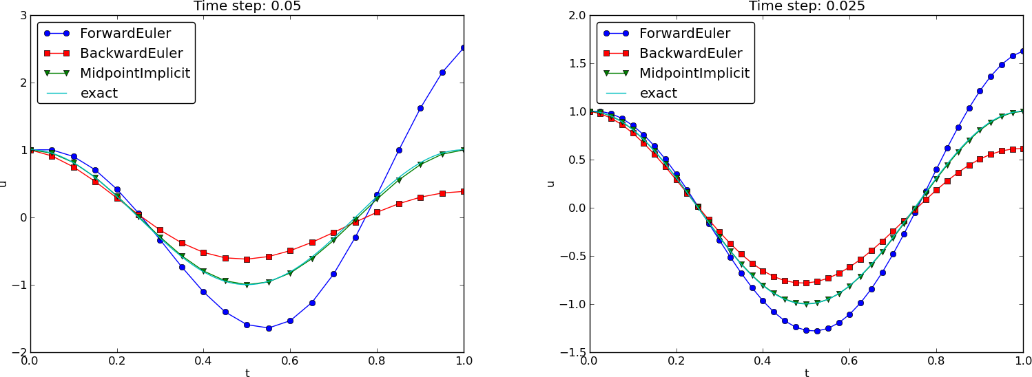
Comparison of classical schemes

We may run two popular standard methods for first-order ODEs, the 2nd- and 4th-order Runge-Kutta methods, to see how they perform. Figures Comparison of Runge-Kutta schemes in the phase plane and Comparison of Runge-Kutta schemes show the solutions with larger \(\Delta t\) values than what was used in the previous two plots.

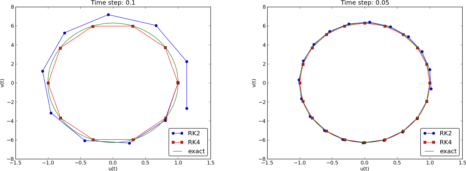
Comparison of Runge-Kutta schemes in the phase plane

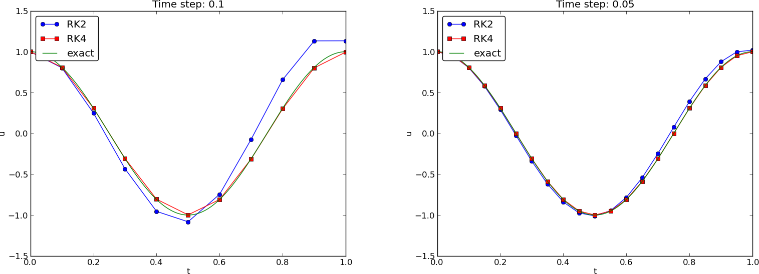
Comparison of Runge-Kutta schemes

The visual impression is that the 4th-order Runge-Kutta method is very accurate, under all circumstances in these tests, and the 2nd-order scheme suffer from amplitude errors unless the time step is very small.

The corresponding results for the Crank-Nicolson scheme are shown in Figures Long-time behavior of the Crank-Nicolson scheme in the phase plane and Long-time behavior of the Crank-Nicolson scheme. It is clear that the Crank-Nicolson scheme outperforms the 2nd-order Runge-Kutta method. Both schemes have the same order of accuracy \({\mathcal{O}(\Delta t^2)}\), but their differences in the accuracy that matters in a real physical application is very clearly pronounced in this example. Exercise 12: Investigate the amplitude errors of many solvers invites you to investigate how

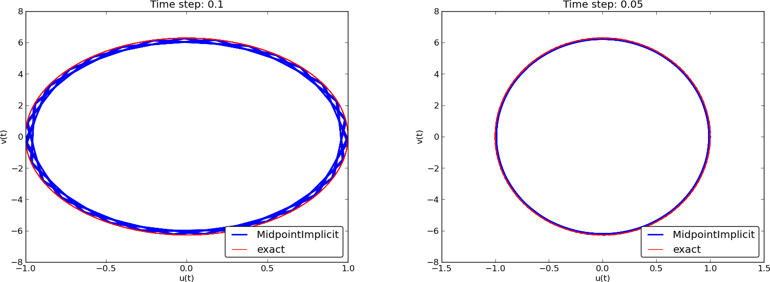
Long-time behavior of the Crank-Nicolson scheme in the phase plane

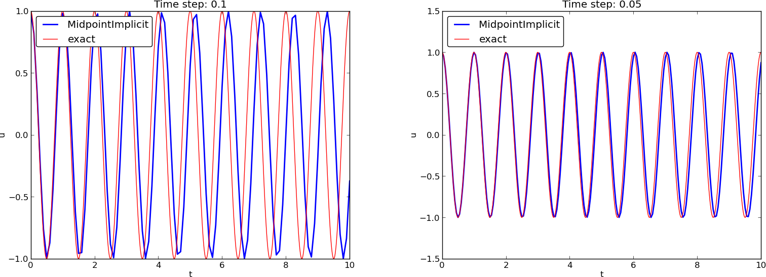
Long-time behavior of the Crank-Nicolson scheme

Enegy considerations

The observations of various methods in the previous section can be better interpreted if we compute an quantity reflecting the total energy of the system. It turns out that this quantity,

\[E(t) = \frac{1}{2}(u')^2 + \frac{1}{2}\omega^2u^2,\]

is constant for all \(t\). Checking that \(E(t)\) really remains constant brings evidence that the numerical computations are sound. Such energy measures, when they exist, are much used to check numerical simulations.

Derivation of the energy expression

We starting multiplying

\[u'' + \omega^2 u = 0,\]

by \(u'\) and integrating from \(0\) to \(T\):

\[\int_0^T u''u' dt + \int_0^T\omega^2 u u' dt = 0{\thinspace .}\]

Observing that

\[u''u' = \frac{d}{dt}\frac{1}{2}(u')^2,\quad uu' = \frac{d}{dt} {\frac{1}{2}}u^2,\]

we get

\[\int_0^T (\frac{d}{dt}\frac{1}{2}(u')^2 + \frac{d}{dt} \frac{1}{2}\omega^2u^2)dt = E(T) - E(0),\]

where we have introduced the energy measure \(E(t)\)

(18)\[ E(t) = \frac{1}{2}(u')^2 + \frac{1}{2}\omega^2u^2{\thinspace .}\]

The important result from this derivation is that the total energy is constant:

\[E(t) = \hbox{const}{\thinspace .}\]

Remark on the energy expression

The quantity \(E(t)\) derived above is physically not the energy of a vibrating mechanical system, but the energy per unit mass. To see this, we start with Newton’s second law \(F=ma\) (\(F\) is the sum of forces, \(m\) is the mass of the system, and \(a\) is the acceleration). The displacement \(u\) is related to \(a\) through \(a=u''\). With a spring force as the only force we have \(F=-ku\), where \(k\) is a spring constant measuring the stiffness of the spring. Newton’s second law then implies the differential equation

\[-ku = mu''\quad\Rightarrow mu'' + ku = 0{\thinspace .}\]

This equation of motion can be turned into an energy balance equation by finding the work done by each term during a time interval \([0,T]\). To this end, we multiply the equation by \(du=u'dt\) and integrate:

\[\int_0^T muu'dt + \int_0^T kuu'dt = 0{\thinspace .}\]

The result is

\[E(t) = E_k(t) + E_p(t) = 0,\]

where

(19)\[ E_k(t) = \frac{1}{}2mv^2,\quad v=u',\]\[is the *kinetic energy* of the system,\]\[ .. _Eq:vib:model1:energy:potential:\]

(20)\[ E_p(t) = {\frac{1}{2}}ku^2\]\[is the *potential energy*, and the sum :math:`E(t)` is the total energy. The derivation demonstrates the famous energy principle that any change in the kinetic energy is due to a change in potential energy and vice versa.\]\[The equation :math:`mu''+ku=0` can be divided by :math:`m` and written as :math:`u'' + \omega^2u=0` for :math:`\omega=\sqrt{k/m}`. The energy expression :math:`E(t)=\frac{1}{2}(u')^2 + \frac{1}{2}\omega^2u^2` derived earlier is then simply the true physical total energy :math:`\frac{1}{2} m(u')^2 + {\frac{1}{2}}k^2u^2` divided by :math:`m`, i.e., total energy per unit mass.\]

Example

Analytically, we have \(u(t)=I\cos\omega t\), if \(u(0)=I\) and \(u'(0)=0\), so we can easily check that the evolution of the energy \(E(t)\) is constant:

\[E(t) = {\frac{1}{2}}I^2 (-\omega\sin\omega t)^2 + \frac{1}{2}\omega^2 I^2 \cos^2\omega t = \frac{1}{2}\omega^2 (\sin^2\omega t + \cos^2\omega t) = \frac{1}{2}\omega^2 {\thinspace .}\]

Discrete total energy

The total energy \(E(t)\) can be computed as soon as \(u^n\) is available. Using \((u')^n\approx [D_{2t} u^n]\) we have

\[E^n = \frac{1}{2}([D_{2t} u]^n)^2 + \frac{1}{2}\omega^2 (u^n)^2{\thinspace .}\]

The errors involved in \(E^n\) get a contribution \({\mathcal{O}(\Delta t^2)}\) from the difference approximation of \(u'\) and a contribution from the numerical error in \(u^n\). With a second-order scheme for computing \(u^n\), the overall error in \(E^n\) is expected to be \({\mathcal{O}(\Delta t^2)}\).

An error measure based on total energy

The error in total energy, as a mesh function, can be computed by

\[e_E^n = \frac{1}{2}\left(\frac{u^{n+1}-u^{n-1}}{2\Delta t}\right)^2 + \frac{1}{2}\omega^2 (u^n)^2 - E(0), \quad n=1,\ldots,N_t-1,\]

where

\[E(0) = {\frac{1}{2}}V^2 + \frac{1}{2}\omega^2I^2,\]

if \(u(0)=I\) and \(u'(0)=V\). A useful norm can be the maximum absolute value of \(e_E^n\):

\[\begin{split}||e_E^n||_{\ell^\infty} = \max_{1\leq n <N_t} |e_E^n|{\thinspace .}\end{split}\]

The corresponding Python implementation takes the form

# import numpy as np and compute u, t
dt = t[1]-t[0]
E = 0.5*((u[2:] - u[:-2])/(2*dt))**2 + 0.5*w**2*u[1:-1]**2
E0 = 0.5*V**2 + 0.5**w**2*I**2
e_E = E - E0
e_E_norm = np.abs(e_E).max()

The convergence rates of the quantity e_E_norm can be used for verification. The value of e_E_norm is also useful for comparing schemes through their ability to preserve energy. Below is a table demonstrating the error in total energy for various schemes. We clearly see that the Crank-Nicolson and 4th-order Runge-Kutta schemes are superior to the 2nd-order Runge-Kutta method and even more superior to the Forward and Backward Euler schemes.

Method	\(T\)	\(\Delta t\)	\(\max \left\vert e_E^n\right\vert\)
Forward Euler	\(1\)	\(0.05\)	\(1.113\cdot 10^{2}\)
Forward Euler	\(1\)	\(0.025\)	\(3.312\cdot 10^{1}\)
Backward Euler	\(1\)	\(0.05\)	\(1.683\cdot 10^{1}\)
Backward Euler	\(1\)	\(0.025\)	\(1.231\cdot 10^{1}\)
Runge-Kutta 2nd-order	\(1\)	\(0.1\)	\(8.401\)
Runge-Kutta 2nd-order	\(1\)	\(0.05\)	\(9.637\cdot 10^{-1}\)
Crank-Nicolson	\(1\)	\(0.05\)	\(9.389\cdot 10^{-1}\)
Crank-Nicolson	\(1\)	\(0.025\)	\(2.411\cdot 10^{-1}\)
Runge-Kutta 4th-order	\(1\)	\(0.1\)	\(2.387\)
Runge-Kutta 4th-order	\(1\)	\(0.05\)	\(6.476\cdot 10^{-1}\)
Crank-Nicolson	\(10\)	\(0.1\)	\(3.389\)
Crank-Nicolson	\(10\)	\(0.05\)	\(9.389\cdot 10^{-1}\)
Runge-Kutta 4th-order	\(10\)	\(0.1\)	\(3.686\)
Runge-Kutta 4th-order	\(10\)	\(0.05\)	\(6.928\cdot 10^{-1}\)

The Euler-Cromer method

While the 4th-order Runge-Kutta method and the a centered Crank-Nicolson scheme work well for the first-order formulation of the vibration model, both were inferior to the straightforward centered difference scheme for the second-order equation \(u''+\omega^2u=0\). However, there is a similarly successful scheme available for the first-order system \(u'=v\), \(v'=-\omega^2u\), to be presented next.

Forward-backward discretization

The idea is to apply a Forward Euler discretization to the first equation and a Backward Euler discretization to the second. In operator notation this is stated as

\[\lbrack D_t^+u = v\rbrack^n,\]

\[\lbrack D_t^-v = -\omega u\rbrack^{n+1} {\thinspace .}\]

We can write out the formulas and collect the unknowns on the left-hand side:

(21)\[ u^{n+1} = u^n + \Delta t v^n,\]

(22)\[ v^{n+1} = v^n -\Delta t \omega^2u^{n+1}\]\[ {\thinspace .}\]

We realize that \(u^{n+1}\) can be computed from (21) and then \(v^{n+1}\) from (22) using the recently computed value \(u^{n+1}\) on the right-hand side.

The scheme (21)-(22) goes under several names: Forward-backward scheme, Semi-implicit Euler method, symplectic Euler, semi-explicit Euler, Newton-Stormer-Verlet, and Euler-Cromer. We shall stick to the latter name. Since both time discretizations are based on first-order difference approximation, one may think that the scheme is only of first-order, but this is not true: the use of a forward and then a backward difference make errors cancel so that the overall error in the scheme is \({\mathcal{O}(\Delta t^2)}\). This is explaned below.

Equivalence with the scheme for the second-order ODE

We may eliminate the \(v^n\) variable from (21)-(22). From (22) we have \(v^n = v^{n-1} - \Delta t \omega^2u^{n}\), which can be inserted in (21) to yield

(23)\[ u^{n+1} = u^n + \Delta t v^{n-1} - \Delta t^2 \omega^2u^{n} .\]

The \(v^{n-1}\) quantity can be expressed by \(u^n\) and \(u^{n-1}\) using (21):

\[v^{n-1} = \frac{u^n - u^{n-1}}{\Delta t},\]

and when this is inserted in (23) we get

\[u^{n+1} = 2u^n - u^{n-1} - \Delta t^2 \omega^2u^{n},\]

which is nothing but the centered scheme (7)! The previous analysis of this scheme then also applies to the Euler-Cromer method. That is, the amplitude is constant, given that the stability criterion is fulfilled, but there is always a phase error (11).

The initial condition \(u'=0\) means \(u'=v=0\). Then \(v^0=0\), and (21) implies \(u^1=u^0\), while (22) says \(v^1=-\omega^2 u^0\). This approximation, \(u^1=u^0\), corresponds to a first-order Forward Euler discretization of the initial condition \(u'(0)=0\): \([D_t^+ u = 0]^0\). Therefore, the Euler-Cromer scheme will start out differently and not exactly reproduce the solution of (7).

The Euler-Cromer scheme on a staggered mesh

The Forward and Backward Euler schemes used in the Euler-Cromer method are both non-symmetric, but their combination yields a symmetric method since the resulting scheme is equivalent with a centered (symmetric) difference scheme for \(u''+\omega^2u=0\). The symmetric nature of the Euler-Cromer scheme is much more evident if we introduce a staggered mesh in time where \(u\) is sought at integer time points \(t_n\) and \(v\) is sought at \(t_{n+1/2}\) between two \(u\) points. The unknowns are then \(u^1, v^{3/2}, u^2, v^{5/2}\), and so on. We typically use the notation \(u^n\) and \(v^{n+\frac{1}{2}}\) for the two unknown mesh functions.

On a staggered mesh it is natural to use centered difference approximations, expressed in operator notation as

\[\lbrack D_t u = v\rbrack^{n+\frac{1}{2}},\]

\[\lbrack D_t v = -\omega u\rbrack^{n+1} {\thinspace .}\]

Writing out the formulas gives

(24)\[ u^{n+1} = u^{n} + \Delta t v^{n+\frac{1}{2}},\]

(25)\[ v^{n+\frac{3}{2}} = v^{n+\frac{1}{2}} -\Delta t \omega^2u^{n+1}\]\[ {\thinspace .}\]

Of esthetic reasons one often writes these equations at the previous time level to replace the \(\frac{3}{2}\) by :math:`frac{1}{2} ` in the left-most term in the last equation,

(26)\[ u^{n} = u^{n-1} + \Delta t v^{n-\frac{1}{2}},\]

(27)\[ v^{n+\frac{1}{2}} = v^{n-\frac{1}{2}} -\Delta t \omega^2u^{n}\]\[ {\thinspace .}\]

Such a rewrite is only mathematical cosmetics. The important thing is that this centered scheme has exactly the same computational structure as the forward-backward scheme. We shall use the names forward-backward Euler-Cromer and staggered Euler-Cromer to distinguish the two schemes.

We can eliminate the \(v\) values and get back the centered scheme based on the second-order differential equation, so all these three schemes are equivalent. However, they differ somewhat in the treatment of the initial conditions.

Suppose we have \(u(0)=I\) and \(u'(0)=v(0)=0\) as mathematical initial conditions. This means \(u^0=I\) and

\[v(0)\approx \frac{1}{2}(v^{-\frac{1}{2}} + v^{\frac{1}{2}}) = 0, \quad\Rightarrow\quad v^{-\frac{1}{2}} =- v^\frac{1}{2}{\thinspace .}\]

Using the discretized equation (27) for \(n=0\) yields

\[v^\frac{1}{2} = v^{-\frac{1}{2}} -\Delta t\omega^2 I,\]

and eliminating \(v^{-\frac{1}{2}} =- v^{\frac{1}{2}}\) results in \(v^\frac{1}{2} = -\frac{1}{2}\Delta t\omega^2I\) and

\[u^1 = u^0 - \frac{1}{2}\Delta t^2\omega^2 I,\]

which is exactly the same equation for \(u^1\) as we had in the centered scheme based on the second-order differential equation (and hence corresponds to a centered difference approximation of the initial condition for \(u'(0)\)). The conclusion is that a staggered mesh is fully equivalent with that scheme, while the forward-backward version gives a slight deviation in the computation of \(u^1\).

We can redo the derivation of the initial conditions when \(u'(0)=V\):

\[v(0)\approx \frac{1}{2}(v^{-\frac{1}{2}} + v^{\frac{1}{2}}) = V, \quad\Rightarrow\quad v^{-\frac{1}{2}} = 2V - v^\frac{1}{2}{\thinspace .}\]

Using this \(v^{-\frac{1}{2}}\) in

\[v^\frac{1}{2} = v^{-\frac{1}{2}} -\Delta t\omega^2 I,\]

then gives \(v^\frac{1}{2} = V - \frac{1}{2}\Delta t\omega^2 I\). The general initial conditions are therefore

(28)\[ u^0 = I,\]

(29)\[ v^\frac{1}{2} = V - \frac{1}{2}\Delta t\omega^2I {\thinspace .}\]

Implementation of the scheme on a staggered mesh

The algorithm goes like this:

1. Set the initial values (28) and (29).
2. For \(n=1,2,\ldots\):

1. Compute \(u^{n}\) from (26).
2. Compute \(v^{n+\frac{1}{2}}\) from (27).

Implementation with integer indices

Translating the schemes (26) and (27) to computer code faces the problem of how to store and access \(v^{n+\frac{1}{2}}\), since arrays only allow integer indices with base 0. We must then introduce a convention: \(v^{1+\frac{1}{2}}\) is stored in v[n] while \(v^{1-\frac{1}{2}}\) is stored in v[n-1]. We can then write the algorithm in Python as

def solver(I, w, dt, T):
    dt = float(dt)
    Nt = int(round(T/dt))
    u = zeros(Nt+1)
    v = zeros(Nt+1)
    t = linspace(0, Nt*dt, Nt+1)  # mesh for u
    t_v = t + dt/2                # mesh for v

    u[0] = I
    v[0] = 0 - 0.5*dt*w**2*u[0]
    for n in range(1, Nt+1):
        u[n] = u[n-1] + dt*v[n-1]
        v[n] = v[n-1] - dt*w**2*u[n]
    return u, t, v, t_v

Note that the return \(u\) and \(v\) together with the mesh points such that the complete mesh function for \(u\) is described by u and t, while v and t_v represents the mesh function for \(v\).

Implementation with half-integer indices

Some prefer to see a closer relationship between the code and the mathematics for the quantities with half-integer indices. For example, we would like to replace the updating equation for v[n] by

v[n+half] = v[n-half] - dt*w**2*u[n]

This is easy to do if we could be sure that n+half means n and n-half means n-1. A possible solution is to define half as a special object such that an integer plus half results in the integer, while an integer minus half equals the integer minus 1. A simple Python class may realize the half object:

class HalfInt:
    def __radd__(self, other):
        return other

    def __rsub__(self, other):
        return other - 1

half = HalfInt()

The __radd__ function is invoked for all expressions n+half (“right add” with self as half and other as n). Similarly, the __rsub__ function is invoked for n-half and results in n-1.

Using the half object, we can implement the algorithms in an even more readable way:

def solver(I, w, dt, T):
    """
    Solve u'=v, v' = - w**2*u for t in (0,T], u(0)=I and v(0)=0,
    by a central finite difference method with time step dt.
    """
    dt = float(dt)
    Nt = int(round(T/dt))
    u = zeros(Nt+1)
    v = zeros(Nt+1)
    t = linspace(0, Nt*dt, Nt+1)  # mesh for u
    t_v = t + dt/2                # mesh for v

    u[0] = I
    v[0+half] = 0 - 0.5*dt*w**2*u[0]
    for n in range(1, Nt+1):
        print n, n+half, n-half
        u[n] = u[n-1] + dt*v[n-half]
        v[n+half] = v[n-half] - dt*w**2*u[n]
    return u, t, v, t_v

Verification of this code is easy as we can just compare the computed u with the u produced by the solver function in vib_undamped.py (which solves \(u''+\omega^2u=0\) directly). The values should coincide to machine precision since the two numerical methods are mathematically equivalent. We refer to the file vib_undamped_staggered.py for the details of a nose test that checks this property.