Note: PRELIMINARY VERSION (expect lots of typos!)
The physical and mathematical problem
The Navier-Stokes equations
Derivation
Boundary conditions
The classical splitting method
A simple, naive approach
A working scheme
Boundary conditions
Spatial discretization by the finite element method
Remark on boundary integrals
Stress formulations
Increasing the implicitness
Methods based on slight compressibility
Fully implicit formulation
Applications
Fluid flow is one of the most common physical phenomena in nature and technological devices. Examples include atmospheric flows ("weather"), global ocean currents, air flow around a car, breathing, and circulation of blood, to mention a few. The focus in the forthcoming text is on a subset of flows without turbulence, where the flow can be considered as incompressible, and where the fluid's viscosity is constant. (Actually, the model to be discussed can be used for turbulence, in principle, but the computations are very heavy.)
For incompressible flow, the key unknowns are the pressure field \( p(\x,t) \) and the velocity field \( \u(\x,t) \). These quantities are governed by the a momentum balance equation,
$$ \begin{equation} \u_t + (\u\cdot\nabla) \u = -\frac{1}{\varrho}\nabla p + \nu\nabla^2\u + \f, \label{ns:NS:mom} \end{equation} $$ and a mass balance equation
$$ \begin{equation} \nabla\cdot\u = 0 \label{ns:NS:mass} \thinspace . \end{equation} $$ Equations \eqref{ns:NS:mom} and \eqref{ns:NS:mass} are known as Navier-Stokes equations for incompressible flow. The parameter \( \varrho \) is the fluid density, \( \nu \) is the (kinematic) viscosity, and \( \f \) denotes body forces such as gravity. Geophysical applications often need to incorporate the Coriolis and centrifugal forces in \( \f \). The Navier-Stokes equations are to be solved in a spatial domain \( \Omega \) for \( t\in (0,T] \).
The derivation of the Navier-Stokes equations contains some equations that are useful for alternative formulations of numerical methods, so we shall briefly recover the steps to arrive at \eqref{ns:NS:mom} and \eqref{ns:NS:mass}. We start with the general momentum balance equation for a continuum (arising from Newton's second law of motion),
$$ \begin{equation} \varrho\Ddt{u} = \nabla\cdot\stress + \varrho\f, \label{ns:momentum:general} \end{equation} $$ where \( \stress \) is the stress tensor and the operator \( D/dt \) is the material derivative, $$ \begin{equation} \Ddt{\u} = \u_t + (\u\cdot\nabla)\u, \end{equation} $$ here denoting acceleration. Therefore, \( \varrho D\u/dt \) is density ("mass") times acceleration, while the terms on the right-hand side are the forces that induce the motion \( \u \): the internal stresses \( \stress \) and the external body forces \( \f \).
The other fundamental equation for a fluid is that of mass conservation, called the continuity equation. It has the general form
$$ \begin{equation} \varrho_t + \nabla\cdot (\varrho\u) = 0, \end{equation} $$ which can be rewritten as $$ \nabla\cdot\u = \frac{1}{\varrho}\Ddt{\varrho} \thinspace. $$ An incompressible flow is defined as a flow where each fluid particle maintains its density. Since \( \Ddt{\varrho} \) is the rate of change of \( \varrho \) of a fluid particle, incompressible flow means \( \Ddt{\varrho}=0 \) and hence \( \nabla\cdot\u = 0 \). The latter is the most useful equation in a PDE system for incompressible flow since it involves the unknown velocity \( \u \).
Different types of fluids will have different relations between the motion \( \u \) and the internal stresses \( \stress \). A Newtonian fluid has an isotropic, linear relation between \( \u \) and \( \stress \):
$$ \begin{equation} \stress = -p\I + \mu (\nabla\u + (\nabla\u)^T), \label{ns:stress:u} \end{equation} $$ where \( \I \) is the identity tensor, and \( \mu \) is the dynamic viscosity (\( \mu = \varrho\nu \)). The relation \eqref{ns:stress:u} assumes incompressible flow. Inserting \eqref{ns:stress:u} in \eqref{ns:momentum:general} gives \eqref{ns:NS:mom} after dividing by \( \varrho \), using \( \nabla\cdot (p\I) = \nabla p \), and calculating \( \nabla\cdot (\nabla\u + (\nabla\u)^T) \) as \( \nabla^2\u + \nabla (\nabla\cdot\u) = \nabla^2\u \). The vector operations involving the nabla operator are easiest performed by using index or dyadic notation, but the derivation of the particular terms is not important for the forthcoming text.
Some numerical methods apply the \( \nabla\cdot\stress = -\nabla p + \nabla\cdot (\nabla\u + (\nabla\u)^T) \) form in \eqref{ns:NS:mom}:
$$ \begin{equation} \u_t + (\u\cdot\nabla) \u = \frac{1}{\varrho}\nabla\cdot\stress + \f, \label{ns:NS:mom:stress0} \end{equation} $$ or $$ \begin{equation} \u_t + (\u\cdot\nabla) \u = -\frac{1}{\varrho}\nabla p + \nu\nabla\cdot (\nabla\u + (\nabla\u)^T) + \f \label{ns:NS:mom:stress} \thinspace . \end{equation} $$
Other formulations add a \( \varrho_t \) term to the continuity equation, usually by assuming slight compressibility. Then \( \varrho = \varrho (p) \) and we have $$ \varrho_t = \frac{\partial\varrho}{\partial p}p_t \thinspace .$$ It is common to evaluate \( \partial\varrho/\partial p \) for some fixed reference value \( \varrho_0 \) so that \( 1/c^2 = \partial\varrho/\partial p \) can be treated as a constant. The parameter \( c \) is the speed of sound in the fluid. The equation of continuity is in such cases often written as
$$ \begin{equation} p_t + c^2\nabla\cdot\u = 0, \label{ns:NS:mass:slightcompr} \end{equation} $$ where we have used the simplification \( \nabla(\varrho\u) = \varrho_0\nabla\u \) for a slightly incompressible fluid and divided the original equation by \( \varrho_0 \).
The incompressible Navier-Stokes equations need three scalar conditions on the velocity components or the stress vector at each point on the boundary. The boundary conditions can be classified as follows.
A combination of velocity and stress boundary conditions at a point is possible. For example, at a symmetry boundary we set the normal velocity to be zero.
The earliest and still the most widely applied numerical method for the incompressible Navier-Stokes equations is based on splitting the PDE system into simpler components for which we can apply standard discretization methods. Such a strategy is known as operator splitting.
The equation \eqref{ns:NS:mom} looks similar to a convection-diffusion equation. The simplest possible numerical method for such equations applies an explicit Forward Euler scheme in time. It is therefore tempting to advance \eqref{ns:NS:mom} in time using a standard Forward Euler discretization:
$$ \begin{equation} \frac{\u^{n+1}-\u^n}{\Delta t} + (\u^n\cdot\nabla)\u^n = -\frac{1}{\varrho} \nabla p^n + \nu\nabla^2\u^n + \f^n, \end{equation} $$ which yields an explicit formula for \( \u^{n+1} \):
$$ \begin{equation} \u^{n+1} = \u^n - \Delta t(\u^n\cdot\nabla)\u^n -\frac{\Delta t}{\varrho} \nabla p^n + \Delta t\,\nu\nabla^2\u^n + \Delta t\f^n \label{ns:split:FE0} \thinspace . \end{equation} $$ There are two fundamental problems with this method:
Intuitively speaking, the fulfillment \( \nabla\cdot\u^{n+1} \) requires us to have "more unknowns to play with" when advancing \eqref{ns:NS:mom}. The idea is to basically use the Forward Euler scheme, but evaluate the pressure term at the new time level \( n+1 \):
$$ \begin{equation} \u^{n+1} = \u^n - \Delta t(\u^n\cdot\nabla)\u^n -\frac{\Delta t}{\varrho} \nabla p^{n+1} + \Delta t\,\nu\nabla^2\u^n + \Delta t\f^n \label{ns:split:FE} \thinspace . \end{equation} $$ We must also require
$$ \begin{equation} \nabla\cdot\u^{n+1} = 0 \thinspace . \label{ns:split:cont} \end{equation} $$ The equations \eqref{ns:split:FE}-\eqref{ns:split:cont} constitute 3+1 coupled PDEs for the 3+1 unknowns \( \u^{n+1} \) and \( p^{n+1} \).
The method for solving \eqref{ns:split:FE}-\eqref{ns:split:cont} is based on a splitting idea where we first propagate the velocity from old values to some intermediate velocity \( \u^* \), using \eqref{ns:split:FE}. Then we enforce the incompressibility constraint \eqref{ns:split:cont} to compute a correction to \( \u^* \) and also the new pressure \( p^{n+1} \).
A plain Forward Euler discretization of \eqref{ns:NS:mom}, but with a weight \( \beta \) on the \( \nabla p^n \) term, reads
$$ \begin{equation} \u^{*} = \u^n - \Delta t(\u^n\cdot\nabla)\u^n - \beta\frac{\Delta t}{\varrho} \nabla p^{n} + \Delta t\,\nu\nabla^2\u^n + \Delta t\f^n \label{ns:split:FE2} \thinspace \end{equation} $$ The intermediate velocity \( \u^* \) does not fulfill the incompressibility constraint \eqref{ns:split:cont}, but we seek a correction \( \delta\u \),
$$ \begin{equation} \u^{n+1} = \u^* + \delta\u, \label{ns:split:corr:du} \end{equation} $$ such that \( \nabla\cdot \u^{n+1} = 0 \). Since \( \delta\u = \u^{n+1} - \u^* \), we can subtract \eqref{ns:split:FE2} from \eqref{ns:split:FE} to find \( \delta\u \).
$$ \begin{equation} \delta\u = \u^{n+1} - \u^* = -\frac{\Delta t}{\varrho}\nabla\Phi \label{ns:split:du} \thinspace . \end{equation} $$ The quantity \( \Phi \) is introduced as a kind of pressure change:
$$ \begin{equation} \Phi = p^{n+1} - \beta p^n \label{ns:split:Phi} \thinspace . \end{equation} $$
Inserting \( \delta\u \) in the incompressibility constraint,
$$ \nabla\cdot (\u^* + \delta\u) = 0,$$ or equivalently, $$ \nabla\cdot\delta\u = - \nabla\cdot \u^* ,$$ results in
$$ \begin{equation} \nabla^2 \Phi = \frac{\varrho}{\Delta t}\nabla\cdot\u^*, \label{ns:split:Poisson} \end{equation} $$ since \( \nabla\cdot\nabla\Phi = \nabla^2\Phi \).
As soon as \( \Phi \) is computed from the Poisson equation \eqref{ns:split:Poisson}, we can calculate
$$ \begin{equation} \u^{n+1} = \u^* -\frac{\Delta t}{\varrho}\nabla\Phi, \label{ns:split:u:np1} \end{equation} $$ and
$$ \begin{equation} p^{n+1} = \Phi + \beta p^n \label{ns:split:p:np1} \thinspace . \end{equation} $$
The solution algorithm at a time level then consists of the following steps:
What boundary conditions should we assign to \( \u^* \) when solving \eqref{ns:split:FE2}? A standard choice is to apply the same boundary conditions as those specified for \( \u \). It follows that \( \delta\u =0 \) on the boundary where \( \u \) is subject to Dirichlet conditions. We let \( \partial\Omega_{D,u} \) denote the part of the boundary \( \partial\Omega \) with Dirichlet conditions, while \( \partial\Omega_{N,u} \) denotes the boundary where Neumann conditions involving \( \partial\u/\partial n \) apply.
The boundary condition on the pressure in the original incompressible Navier-Stokes equations is simply to prescribe \( p \) at a single point, potentially as a function of time. However, when solving the Poisson equation \eqref{ns:split:Poisson} we need Dirichlet or Neumann boundary conditions for \( \Phi \) (the pressure change) on the whole boundary. Sometimes the pressure is prescribed at an inlet or outlet boundary, which then yields a Dirichlet condition for \( \Phi = p^{n+1}-\beta p^n \). At the boundaries where \( \u \) is subject to Dirichlet conditions, \( \u^* \) has the same conditions, and \( \delta\u = 0 \), which implies \( \nabla\Phi =0 \). In particular, \( \partial\Phi/\partial n=0 \), and homogeneous Neumann conditions are therefore used on such boundaries when solving the Poisson equation for \( \Phi \). Also, at symmetry boundaries, \( \partial\Phi/\partial n=0 \). At an inlet boundary, a pressure gradient in the flow direction is often known, say as \( f(t) \), implying that we can compute \( \partial\Phi/\partial n= -(f(t^{n+1}) - \beta f(t^n)) \).
We let \( \partial\Omega_{D,\Phi} \) be the part of the boundary where \( \Phi \) is subject to Dirichlet conditions, while \( \partial\Omega_{N,p} \) is the remaining part where Neumann conditions involving \( \partial\Phi/\partial n \) are assigned.
The equations to be solved, \eqref{ns:split:FE2}, \eqref{ns:split:Poisson}, \eqref{ns:split:u:np1}, and \eqref{ns:split:p:np1}, are of two types: explicit updates (approximations a la \( u=f \)) and the Poisson equation. We introduce a vector test function \( \v^{(u)}\in V^{(u)} \) for the vector equations \eqref{ns:split:FE2} and \eqref{ns:split:u:np1}, and a scalar test function \( v^{(\Phi)}\in V^{(\Phi)} \) for the Poisson equation and the update \eqref{ns:split:p:np1}. Modulo nonzero Dirichlet conditions, we seek \( \u^*,\u^{n+1}\in V^{(u)} \) and \( p^{n+1}\in V^{(\Phi)} \).
The variational form of a vector equation like \eqref{ns:split:FE2} is derived by taking the inner product of the equation and \( \v^{(u)} \). The Laplace term is integrated by parts, as usual, but this time vectors are involved. The relevant rule takes the form
$$ \int_\Omega (\nabla^2\u )\cdot\v\dx = -\int_\Omega \nabla\u :\nabla v\dx + \int_{\partial\Omega}\frac{\partial\u}{\partial n}\cdot\v \ds,$$ where \( \nabla\u :\nabla\v \) means the inner tensor product: \( \pmb{A}:\pmb{B} = \sum_j\sum_j A_{ij}B_{ij} \) (when \( \pmb{A} \) has elements \( A_{i,j} \) and \( \pmb{B} \) has elements \( B_{i,j} \). Alternatively, we may say that \( \pmb{A}:\pmb{B} \) is simply the scalar product of the tensors \( \pmb{A} \) and \( \pmb{B} \) when these are viewed as vectors (of length 9 instead of tensors of dimension \( 3\times 3 \) in 3D problems). The normal derivative has the usual definition: \( \partial\u/\partial n = \normalvec\cdot \nabla\u \).
The \( \int_\Omega \nabla p^n\cdot\v^{(u)}\dx \) integral can also be a candidate for integrated by parts, if desired. The relevant rule reads
$$ \int_\Omega \nabla p\cdot\v \dx = -\int_\Omega p\nabla\cdot\v\dx + \int_{\partial\Omega} p\normalvec\cdot\v\ds\thinspace .$$ We use such an integration by parts below. The advantage is that we get a boundary integral involving \( p\normalvec \), which is advantageous if we want to set a condition on \( p \), especially at an outflow boundary, but also on an inflow boundary.
For notational simplicity and close correspondence to computer code, we introduce the subscript 1 on quantities from the previous time level \( n \) and drop any superscript \( n+1 \) for quantities to be computed at the new time level. The resulting variational form can be written as
$$ \begin{align} & \int_\Omega \bigl( \u^*\cdot\v^{(u)} + \Delta t((\u_1\cdot\nabla)\nabla\u_1)\cdot\v^{(u)} - \frac{\Delta t}{\varrho}p\nabla\cdot\v^{(u)} + \nonumber\\ & \Delta t\,\nu\nabla\u_1 : \nabla\v^{(u)} - \Delta t f_1\bigr)\dx = \int_{\partial\Omega_{N,u}}\left( \nu\frac{\partial\u}{\partial n} - p\normalvec\right)\cdot\v^{(u)}\ds, \label{ns:split:FE2:vf} \end{align} $$ \( \forall\v^{(u)}\in V^{(u)} \). The variational form corresponding to the Poisson equation becomes
$$ \begin{equation} \int_\Omega\nabla\Phi\cdot\nabla v^{(\Phi)}\dx = - \frac{\varrho}{\Delta t}\int_\Omega \nabla\cdot\u^*\, v^{(\Phi)}\dx + \int_{\partial\Omega_{N,p}} \frac{\partial\Phi}{\partial n}v^{(\Phi)}\ds, \quad\forall v^{(\Phi)}\in V^{(\Phi)} \thinspace . \label{ns:split:Poisson:vf} \end{equation} $$
The variational form for the velocity update \eqref{ns:split:u:np1} is based on taking the inner product of \( \v^{(u)} \) and \eqref{ns:split:u:np1}:
$$ \begin{equation} \int_\Omega \u\cdot\v^{(u)}\dx = \int_{\Omega} (\u^* -\frac{\Delta t}{\varrho} \nabla\Phi)\cdot\v^{(u)}\dx,\quad\forall\v^{(u)}\in V^{(u)} \thinspace . \label{ns:split:u:np1:vf} \end{equation} $$ Note that this is the same form as in a vector approximation problem: approximate a given vector field \( \f \) by a \( \u \), where the components of \( \u \) are scalar finite element functions. Also note that \( \u \) in \eqref{ns:split:u:np1:vf} is actually \( \u^{n+1} \), but that the superscript is dropped since we do not use that in an implementation.
The pressure update has the variational form
$$ \begin{equation} \int_\Omega p v^{(\Phi)}\dx = \int_{\Omega} (\Phi + \beta p_1)v^{(\Phi)}\dx, \quad\forall v^{(\Phi)}\in V^{(\Phi)} \thinspace . \label{ns:split:p:np1:vf} \end{equation} $$ (Also here, \( p \) denotes \( p^{n+1} \) and \( p_1 \) is \( p^n \).)
The splitting method presented above allows flexible choices of elements for \( \u \) and \( p \). In the early days of the finite element method for incompressible flow, fully implicit formulations were used and these require the \( \u \) element to be of one polynomial degree higher than the \( p \) element. This restriction does not apply to the splitting scheme, so one may, e.g., choose P1 elements for the velocity components and the pressure.
The boundary integral in \eqref{ns:split:FE2:vf} comes into play at element faces on the boundary if the nodes on a face are not subject to Dirichlet conditions. As for scalar PDEs, Dirichlet conditions either mean that \( \v=0 \) on that part of the boundary, or the element matrix and vector (or the global coefficient matrix and right-hand side) are manipulated to enforce known values of the unknown such that any boundary integral is erased and replaced by the boundary value.
The boundary integral most often applies to inflow and outflow boundaries \( x=\hbox{const} \) where we assume unidirectional flow, \( \u = u\ii \). Because of \( \nabla\cdot\u = 0 \) we have \( \partial\u/\partial x = \partial\u/\partial n=0 \) and \( p=\hbox{const} \). Very often, the boundary integral in \eqref{ns:split:FE2:vf} is zero, because we apply it to an outflow boundary where we have \( \partial\u/\partial n=0 \) and then we fix the pressure at \( p=0 \). Note that in the original Navier-Stokes equations, \( p \) enters just through \( \nabla p \) so a boundary condition at one point is necessary to uniquely determine \( p \) (otherwise \( p \) is known up to a free additive constant). At inflow boundaries, \( \u \) is either known, which implies that the boundary integral does not apply, or we have \( \partial\u/\partial n=0 \) and \( p=p_0 \). In this latter case, the boundary integral involves an integration of \( p\normalvec\cdot\v \).
The boundary integral involving \( \partial\Phi/\partial n \) is usually omitted since we apply the condition \( \partial\Phi/\partial n =0 \), see the section Boundary conditions.
As mentioned in the section Derivation, we may exchange the \( \nu\nabla^2\u \) term in \eqref{ns:NS:mom} with a stress term \( \varrho^{-1}\nabla\cdot\stress \), where \( \stress \) is given by \eqref{ns:stress:u}. Occasionally, the \( \nabla\cdot\stress \) term is advantageous, because integration by parts of \( \int_\Omega\nabla\cdot\stress\cdot\v^{(u)}\dx \) gives a boundary integral with the stress vector \( \stress\cdot\normalvec \). This is convenient when boundary conditions are formulated in terms of stresses.
The explicit scheme \eqref{ns:split:FE2} resembles the same stability problems as when a Forward Euler scheme is applied to the diffusion equation. However, there is also a convection term \( \u\cdot\nabla\u \) that reduces the time step restrictions. The stability criterion reads
$$ \begin{equation} \Delta t \leq \frac{h^2}{2\nu + Uh}, \end{equation} $$ where \( h \) is the minimum element size and \( U \) is a characteristic size of the velocity. The term \( 2\nu \) stems from the viscous (Laplace) term while \( Uh \) arises from the convection term in the Navier-Stokes equations. Which of the term that dominates in the denominator therefore depends on whether viscous forces or convection is important in the equation.
Treating the viscosity term \( \nu\nabla^2\u \) implicitly helps greatly on the stability properties of the scheme for \( \u^* \). We may, for example, apply a Backward Euler scheme. Instead of \eqref{ns:split:FE} we then have
$$ \begin{align} \u^{n+1} &= \u^n - \Delta t(\u^{n+1}\cdot\nabla)\u^{n+1} -\frac{\Delta t}{\varrho} \nabla p^{n+1} + \Delta t\,\nu\nabla^2\u^{n+1} + \Delta t\f^{n+1}, \label{ns:split:BE}\\ \nabla\cdot\u^{n+1} &= 0 \thinspace . \end{align} $$ An intermediate velocity can be computed from the first equation if we replace \( p^{n+1} \) by \( \beta p^n \) as done earlier:
$$ \u^{*} = \u^n - \Delta t(\u^{*}\cdot\nabla)\u^{*} - \beta\frac{\Delta t}{\varrho} p^{n+1} + \Delta t\,\nu\nabla^2\u^{*} + \Delta t\f^{n+1} \label{ns:split:BE1} \thinspace $$ To simplify the nonlinearity in \( (\u^{*}\cdot\nabla)\u^{*} \) we may use an old value in the convective velocity:
$$ \begin{equation} (\u^{*}\cdot\nabla)\u^{*} \approx (\u^{n}\cdot\nabla)\u^{*} \thinspace . \end{equation} $$ This approximation is essentially one Picard iteration using \( u^n \) as initial guess.
The intermediate velocity \( \u^* \) is now governed by a linear problem
$$ \u^{*} = \u^n - \Delta t(\u^{n}\cdot\nabla)\u^{*} - \beta\frac{\Delta t}{\varrho} \nabla p^{n} + \Delta t\,\nu\nabla^2\u^{*} + \Delta t\f^{n+1} \label{ns:split:BE2} \thinspace $$ The correction \( \delta\u = \u^{n+1} - \u^* \) becomes
$$ \delta\u = \Delta t((\u^{n+1}\cdot\nabla)\u^{n+1} - (\u^{n}\cdot\nabla)\u^{*}) -\frac{\Delta t}{\varrho} \nabla \Phi + \Delta t\,\nu (\nabla^2 (\u^{n+1} - \u^*) \thinspace .$$ Under the assumption that \( \u^* \) is close to \( \u^{n+1} \), we may drop the terms involving \( \u^{n+1}-\u^* \) and just keep the \( \nabla\Phi \) term. Then
$$ \delta\u = \u^{n+1} - \u^* = -\frac{\Delta t}{\varrho}\nabla\Phi, $$ as before, and the incompressibility constraint \( \nabla\cdot\delta\u = - \nabla\cdot\u^* \) gives \( \nabla^2 \Phi = \frac{\varrho}{\Delta t}\nabla\cdot\u^* \).
The algorithm becomes the same as for a Forward Euler discretization, except that \eqref{ns:split:FE2} is replaced by \eqref{ns:split:BE2}.
By allowing a slight compressibility we can replace the problematic constraint \( \nabla\cdot\u \) by an evolution equation \eqref{ns:NS:mass:slightcompr} for \( p \). Essentially, we then have two evolution equations for \( \u \) and \( p \):
$$ \begin{align} \u_t &= -(\u\cdot\nabla) \u -\frac{1}{\varrho}\nabla p + \nu\nabla^2\u + \f,\\ p_t &= - c^2\nabla\cdot\u \thinspace . \end{align} $$ The simplest method is a Forward Euler scheme:
$$ \begin{align} \u^{n+1} &= \u^n - \Delta t (\u^n\cdot\nabla) \u^n -\frac{\Delta t}{\varrho}\nabla p^n + \Delta t\,\nu\nabla^2\u^n + \Delta t\f^n,\\ p^{n+1} &= p^n - \Delta t c^2\nabla\cdot\u^n \thinspace . \end{align} $$ The major problem with this scheme is the stability constraint, which is dictated by the \( c \) parameter (velocity of sound): \( \Delta t \sim 1/c \). Usually, \( c \) is taken as a tuning parameter and values much less than the speed of sound may give solutions with acceptable compressibility.
Any other explicit scheme, say a 2nd- or 4th-order Runge-Kutta method, is easily applied. Implicit schemes are of course also possible, but then one has to solve linear systems, and the original formulation with a true incompressibility constraint \( \nabla\cdot\u = 0 \) is not more complicated and usually preferred. In general, the method based on slight compressibility and explicit time integration becomes computationally very heavy and is not competitive unless one can use a \( c \) value much lower than the speed of sound.
Early attempts to use the finite element method to solve the Navier-Stokes equations were based on fully implicit formulations. This is easily derived by applying a Backward Euler scheme to the system \eqref{ns:NS:mom}-\eqref{ns:NS:mass}:
$$ \begin{align*} \frac{\u^n - \u^{n-1}}{\Delta t} + (\u^n\cdot\nabla) \u^n &= -\frac{1}{\varrho}\nabla p^n + \nu\nabla^2\u^n + \f^n,\\ \nabla\cdot\u^n &= 0 \end{align*} $$ We introduce the test functions \( \v^{(u)}\in V^{(u)} \) for the momentum balance equation and seek \( \u^{n+1}\in V^{(u)} \) (or more precisely, the part of \( \u^{n+1} \) without nonzero Dirichlet conditions). We seek \( p\in V^{(p)} \) and use \( v^{(p}\in V^{(p} \) as test function for the continuity equation. We may write the system of PDEs as
$$ \begin{align*} {\cal L}_u (\u^{n}, p^{n}, \u^{n-1}) &= 0,\\ \nabla\cdot\u^n &= 0\thinspace . \end{align*} $$ A variational formulation can be based on treating the two equations separately,
$$ \begin{align*} \int_\Omega {\cal L}_u (\u^{n}, p^{n}, \u^{n-1})\cdot\v^{(u)}\dx &= 0,\\ \int_\Omega \nabla\cdot\u^n v^{(p)}\dx &= 0, \end{align*} $$ or we may use an inner product of the two equations \( ({\cal L}_u, \nabla\cdot\u) \) and the test vector \( (\v^{(u)}, v^{(p)}) \):
$$ \int_\Omega \left( {\cal L}_u (\u^{n}, p^{n}, \u^{n-1})\cdot\v^{(u)} + \nabla\cdot\u^n v^{(p)}\right)\dx = 0\thinspace . $$ To minimize the distance between code and mathematics, we introduce new symbols: \( \u \) for \( \u^n \), \( \u_1 \) for \( \u^{n-1} \), and \( p \) for \( p^n \). Integrating the pressure and viscous terms by parts yields
$$ \begin{align} \int_\Omega \bigl( \u \cdot\v^{(u)} &+ \Delta t((\u \cdot\nabla)\nabla\u )\cdot\v^{(u)} - \frac{\Delta t}{\varrho}p\nabla\cdot\v^{(u)} + \nonumber\\ & \Delta t\,\nu\nabla\u\cdot\nabla\v^{(u)} - \Delta t f\bigr)\dx + \int_{\partial\Omega_{N,u}}\left( \nu\frac{\partial\u}{\partial n} - p\normalvec\right)\cdot\v^{(u)}\ds + \nonumber \\ & \int_{\Omega} \nabla\cdot\u\, v^{(p)}\dx = 0 \thinspace . \label{ns:fullyimpl:BE:vf} \end{align} $$ This is nothing but a coupled, nonlinear equation system for \( \u \) and \( p \). Inserting finite element expansions for \( \u \) and \( p \) yields discrete equations that can be written in matrix form as
$$ \begin{align} Mu + \Delta t C(u)u &= -\frac{\Delta t}{\varrho} Lp + \nu Kp + f,\\ L^T u &= 0, \end{align} $$ where \( M \) is the usual mass matrix, but here for a vector function, \( u \) collects all coefficients for the \( \u \) field, \( C(u) \) is a matrix arising from the convection term \( (\u\cdot\nabla)\u \), \( L \) is a matrix arising from the \( p\nabla\cdot\v^{(u)} \) term, \( K \) is the matrix corresponding to the Laplace operator (acting on a vector), and \( f \) is a vector of the source terms arising from \( \f \). The nonlinearity is typically handled by a Newton method.
The simplified system arising from dropping the time derivative and the convection term \( (\u\cdot\nabla)\u \) can be analyzed. It turns out that only certain combinations of \( V^{(u)} \) and \( V^{(p)} \) can guarantee a stable solution. The polynomials in \( V^{(u)} \) must be (at least) one degree higher than those in \( V^{(p)} \). For example, one may use P2 elements for \( \u \) and P1 elements for \( p \). This combination is known as the famous Taylor-Hood element. Numerical experimentation indicates that the same stability restriction on the combination of spaces is also important for the fully nonlinear Navier-Stokes equations when solved by a fully implicit method. The splitting into simpler systems, as shown in the section A working scheme, introduces further approximations that stabilize the problem such that the same type of element can be used for velocity components and pressure.
The splitting method is much more widely used than the fully implicit formulation. Although the latter is more robust and much better suited for stationary flow, it is also involves much heavier computations. In each Newton iteration, a linear system involving all the coefficients in \( \u \) and \( p \) must be solved, and it is non-trivial to construct efficient iterative solution methods (especially preconditioners).
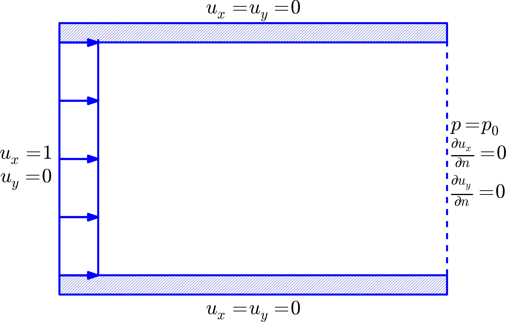
Figure 1 exemplifies the boundary conditions for flow in a channel between two infinite plates. This flow configuration is assumed to be stationary, \( \u_t=0 \), and a simple analytical solution can be found in this particular case.
Note that the numerical solution method described above requires a time-dependent problem. Stationary problems must be simulated by starting with some initial condition and letting the flow develop toward the stationary solution as \( t\rightarrow\infty \).
The velocity field in channel flow is symmetric with respect to the center line. It is therefore sufficient to calculate the flow in half the channel. Figure 2 displays the computational domain and the relevant boundary conditions.
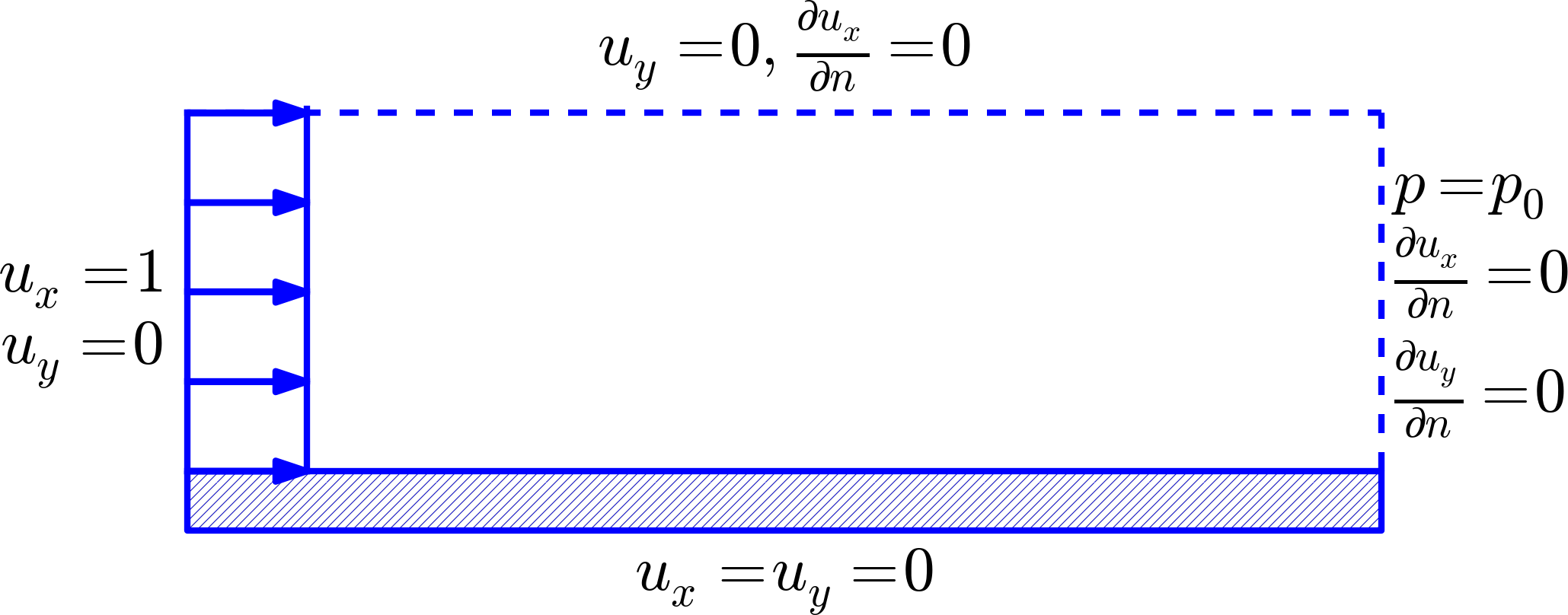
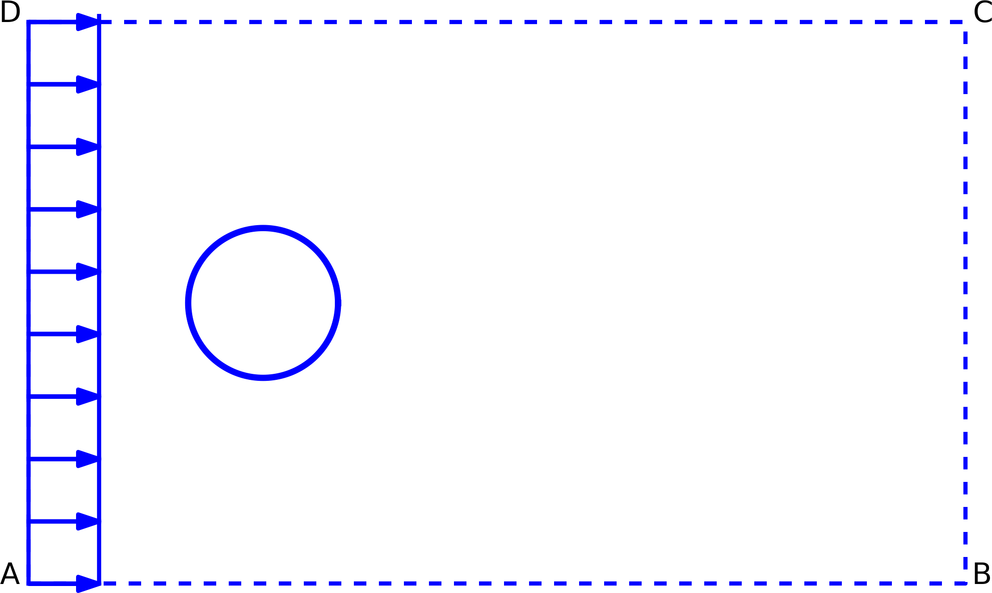
Figure 3 depicts a more complex flow geometry, leading to a more complex velocity field. The boundary conditions are, however, similar to those for channel flow.

The boundary conditions in Figure 4 are not listed in the figure because there are multiple options. The inflow boundary must have a prescribed velocity \( \u \), and on the cylinder we must have \( \u = 0 \). On the remaining three boundaries we have some freedom in what to assign. At the outflow one typically sets \( \partial\u/\partial n=0 \) and fix the pressure at one value. Alternatively, one may apply a stress-free condition \( \stress\cdot\normalvec = 0 \), which implicitly also sets the pressure. On the boundaries AB and DC there is more freedom. The weakest condition is \( \partial\u/\partial n=0 \), assuming that the boundary is far enough away from the cylinder such that the flow field changes very little. Some prefer to set \( \stress\cdot\normalvec = 0 \) here instead. A stronger condition is to require \( u_y=0 \) and \( \partial u_x/\partial n=0 \). However, \( u_y=0 \) requires the boundary to be far away from the cylinder.