Study Guide: Finite difference methods for vibration problems

Table of contents

A simple vibration problem
      A centered finite difference scheme; step 1 and 2
      A centered finite difference scheme; step 3
      A centered finite difference scheme; step 4
      Computing the first step
      The computational algorithm
      Operator notation; ODE
      Operator notation; initial condition
      Computing \( u' \)
Implementation
      Core algorithm
      Plotting
      Main program
      User interface: command line
      Running the program
Verification
      First steps for testing and debugging
      Checking convergence rates
      Implementational details
      Nose test
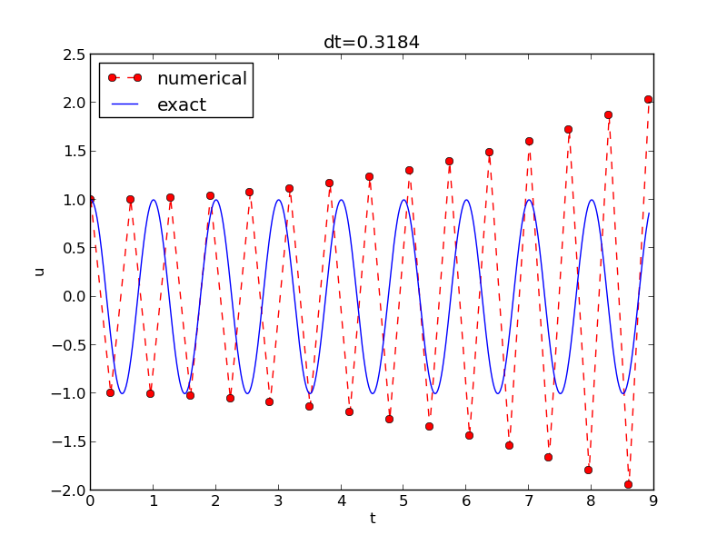
Long time simulations
      Effect of the time step on long simulations
      Using a moving plot window
Analysis of the numerical scheme
      Deriving an exact numerical solution; ideas
      Deriving an exact numerical solution; calculations (1)
      Deriving an exact numerical; calculations (2)
      Polynomial approximation of the phase error
      Plot of the phase error
      Exact discrete solution
      Convergence of the numerical scheme
      Stability
      The stability criterion
      Summary of the analysis
Alternative schemes based on 1st-order equations
      Rewriting 2nd-order ODE as system of two 1st-order ODEs
      The Forward Euler scheme
      The Backward Euler scheme
      The Crank-Nicolson scheme
      Comparison of schemes via Odespy
      Forward and Backward Euler and Crank-Nicolson
      Phase plane plot of the numerical solutions
      Plain solution curves
      Observations from the figures
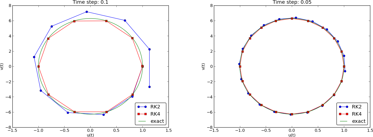
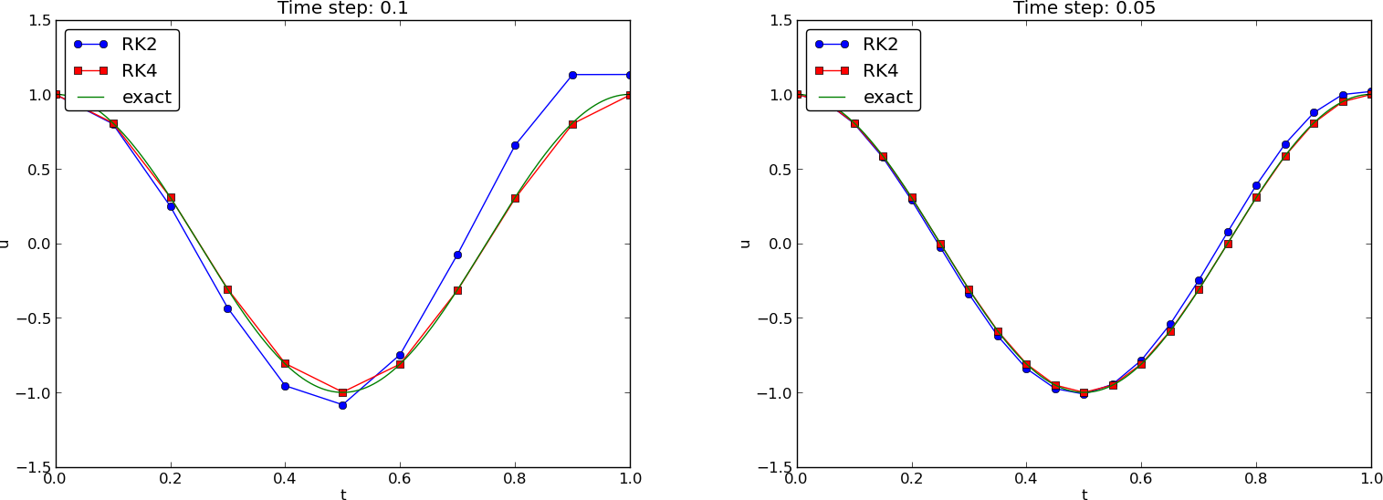
      Runge-Kutta methods of order 2 and 4; short time series
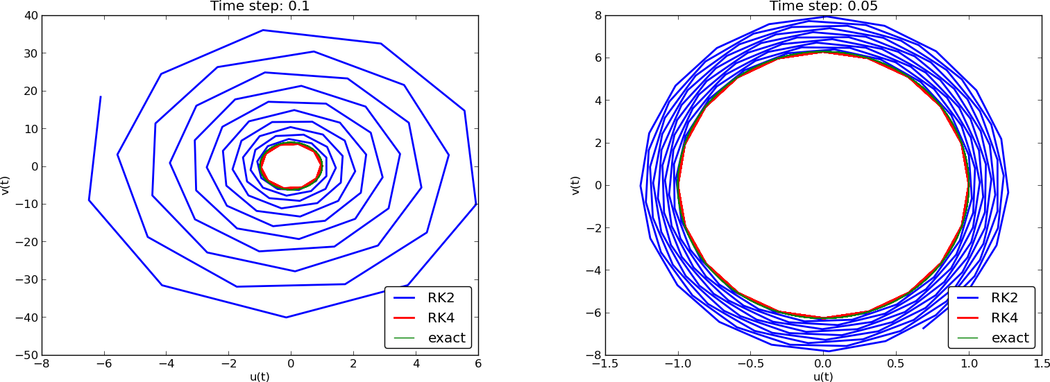
      Runge-Kutta methods of order 2 and 4; longer time series
      Crank-Nicolson; longer time series
      Observations of RK and CN methods
      Energy conservation property
      Derivation of the energy conservation property
      Remark about \( E(t) \)
      The Euler-Cromer method; idea
      The Euler-Cromer method; complete formulas
      Equivalence with the scheme for the second-order ODE
      Comparison of the treatment of initial conditions
      A method utilizing a staggered mesh
      Centered differences on a staggered mesh
      Comparison with the scheme for the 2nd-order ODE
      Implementation of a staggered mesh; integer indices
      Implementation of a staggered mesh; half-integer indices (1)
      Implementation of a staggered mesh; half-integer indices (2)
Generalization: damping, nonlinear spring, and external excitation
      A centered scheme for linear damping
      Initial conditions
      Linearization via a geometric mean approximation
      A centered scheme for quadratic damping
      Initial condition for quadratic damping
      Algorithm
      Implementation
      Verification
      Demo program
      Euler-Cromer formulation
      Staggered grid
      Linear damping
      Quadratic damping
      Initial conditions

A simple vibration problem

$$ \begin{equation} u''t + \omega^2u = 0,\quad u(0)=I,\ u'(0)=0,\ t\in (0,T] \tp \label{vib:model1} \end{equation} $$

Exact solution:

$$ \begin{equation} u(t) = I\cos (\omega t) \tp \label{vib:model1:uex} \end{equation} $$ \( u(t) \) oscillates with constant amplitude \( I \) and (angular) frequency \( \omega \). Period: \( P=2\pi/\omega \).

A centered finite difference scheme; step 1 and 2

• Strategy: follow the four steps of the finite difference method.
• Step 1: Introduce a time mesh, here uniform on \( [0,T] \): \( t_n=n\Delta t \)
• Step 2: Let the ODE be satisfied at each mesh point:

A centered finite difference scheme; step 3

Step 3: Approximate derivative(s) by finite difference approximation(s). Very common (standard!) formula for \( u'' \):

$$ \begin{equation} u''(t_n) \approx \frac{u^{n+1}-2u^n + u^{n-1}}{\Delta t^2} \tp \label{vib:model1:step3} \end{equation} $$

Use this discrete initial condition together with the ODE at \( t=0 \) to eliminate \( u^{-1} \) (insert \eqref{vib:model1:step3} in \eqref{vib:model1:step2}):

$$ \begin{equation} \frac{u^{n+1}-2u^n + u^{n-1}}{\Delta t^2} = -\omega^2 u^n \tp \label{vib:model1:step4a} \end{equation} $$

A centered finite difference scheme; step 4

Step 4: Formulate the computational algorithm. Assume \( u^{n-1} \) and \( u^n \) are known, solve for unknown \( u^{n+1} \):

$$ \begin{equation} u^{n+1} = 2u^n - u^{n-1} - \Delta t^2\omega^2 u^n \tp \label{vib:model1:step4} \end{equation} $$

Nick names for this scheme: Stormer's method or Verlet integration.

Computing the first step

• The formula breaks down for \( u^1 \) because \( u^{-1} \) is unknown and outside the mesh!
• And: we have not used the initial condition \( u'(0)=0 \).

Inserted in \eqref{vib:model1:step4} for \( n=0 \) gives

$$ \begin{equation} u^1 = u^0 - \half \Delta t^2 \omega^2 u^0 \tp \label{vib:model1:step4b} \end{equation} $$

The computational algorithm

1. \( u^0=I \)
2. compute \( u^1 \) from \eqref{vib:model1:step4b}
3. for \( n=1,2,\ldots,N_t-1 \):

1. compute \( u^{n+1} \) from \eqref{vib:model1:step4}

t = linspace(0, T, Nt+1)  # mesh points in time
dt = t[1] - t[0]          # constant time step.
u = zeros(Nt+1)           # solution

u[0] = I
u[1] = u[0] - 0.5*dt**2*w**2*u[0]
for n in range(1, Nt):
    u[n+1] = 2*u[n] - u[n-1] - dt**2*w**2*u[n]

Note: w is consistently used for \( \omega \) in my code.

Operator notation; ODE

With \( [D_tD_t u]^n \) as the finite difference approximation to \( u''(t_n) \) we can write

$$ \begin{equation} [D_tD_t u + \omega^2 u = 0]^n \tp \label{vib:model1:step4:op} \end{equation} $$

\( [D_tD_t u]^n \) means applying a central difference with step \( \Delta t/2 \) twice:

$$ [D_t(D_t u)]^n = \frac{[D_t u]^{n+\half} - [D_t u]^{n-\half}}{\Delta t}$$ which is written out as $$ \frac{1}{\Delta t}\left(\frac{u^{n+1}-u^n}{\Delta t} - \frac{u^{n}-u^{n-1}}{\Delta t}\right) = \frac{u^{n+1}-2u^n + u^{n-1}}{\Delta t^2} \tp $$

Operator notation; initial condition

$$ \begin{equation} [u = I]^0,\quad [D_{2t} u = 0]^0, \end{equation} $$ where \( [D_{2t} u]^n \) is defined as $$ \begin{equation} [D_{2t} u]^n = \frac{u^{n+1} - u^{n-1}}{2\Delta t} \tp \end{equation} $$

Computing \( u' \)

\( u \) is often displacement/position, \( u' \) is velocity and can be computed by

$$ \begin{equation} u'(t_n) \approx \frac{u^{n+1}-u^{n-1}}{2\Delta t} = [D_{2t}u]^n \tp \end{equation} $$

Implementation

Core algorithm

from numpy import *
from matplotlib.pyplot import *
from vib_empirical_analysis import minmax, periods, amplitudes

def solver(I, w, dt, T):
    """
    Solve u'' + w**2*u = 0 for t in (0,T], u(0)=I and u'(0)=0,
    by a central finite difference method with time step dt.
    """
    dt = float(dt)
    Nt = int(round(T/dt))
    u = zeros(Nt+1)
    t = linspace(0, Nt*dt, Nt+1)

    u[0] = I
    u[1] = u[0] - 0.5*dt**2*w**2*u[0]
    for n in range(1, Nt):
        u[n+1] = 2*u[n] - u[n-1] - dt**2*w**2*u[n]
    return u, t

Plotting

def exact_solution(t, I, w):
    return I*cos(w*t)

def visualize(u, t, I, w):
    plot(t, u, 'r--o')
    t_fine = linspace(0, t[-1], 1001)  # very fine mesh for u_e
    u_e = exact_solution(t_fine, I, w)
    hold('on')
    plot(t_fine, u_e, 'b-')
    legend(['numerical', 'exact'], loc='upper left')
    xlabel('t')
    ylabel('u')
    dt = t[1] - t[0]
    title('dt=%g' % dt)
    umin = 1.2*u.min();  umax = -umin
    axis([t[0], t[-1], umin, umax])
    savefig('vib1.png')
    savefig('vib1.pdf')
    savefig('vib1.eps')

Main program

I = 1
w = 2*pi
dt = 0.05
num_periods = 5
P = 2*pi/w    #  one period
T = P*num_periods
u, t = solver(I, w, dt, T)
visualize(u, t, I, w, dt)

User interface: command line

import argparse
parser = argparse.ArgumentParser()
parser.add_argument('--I', type=float, default=1.0)
parser.add_argument('--w', type=float, default=2*pi)
parser.add_argument('--dt', type=float, default=0.05)
parser.add_argument('--num_periods', type=int, default=5)
a = parser.parse_args()
I, w, dt, num_periods = a.I, a.w, a.dt, a.num_periods

Running the program

vib_undamped.py:

Terminal> python vib_undamped.py --dt 0.05 --num_periods 40

Generates frames tmp_vib%04d.png in files. Can make movie:

Terminal> avconv -r 12 -i tmp_vib%04d.png -vcodec flv movie.flv

Can use ffmpeg instead of avconv.

Verification

First steps for testing and debugging

• Testing very simple solutions: \( u=\hbox{const} \) or \( u=ct + d \) do not apply here (without a force term in the equation: \( u'' + \omega^2u = f \)).
• Hand calculations: calculate \( u^1 \) and \( u^2 \) and compare with program.

Checking convergence rates

The next function estimates convergence rates, i.e., it

• performs \( m \) simulations with halved time steps: \( 2^{-k}\Delta t \), \( k=0,\ldots,m-1 \),
• computes the \( L_2 \) norm of the error, \( E = \sqrt{\Delta t_i\sum_{n=0}^{N_t-1}(u^n-\uex(t_n))^2} \) in each case,
• estimates the rates \( r_i \) from two consecutive experiments \( (\Delta t_{i-1}, E_{i-1}) \) and \( (\Delta t_{i}, E_{i}) \), assuming \( E_i=C\Delta t_i^{r_i} \) and \( E_{i-1}=C\Delta t_{i-1}^{r_i} \):

Implementational details

def convergence_rates(m, num_periods=8):
    """
    Return m-1 empirical estimates of the convergence rate
    based on m simulations, where the time step is halved
    for each simulation.
    """
    w = 0.35; I = 0.3
    dt = 2*pi/w/30  # 30 time step per period 2*pi/w
    T = 2*pi/w*num_periods
    dt_values = []
    E_values = []
    for i in range(m):
        u, t = solver(I, w, dt, T)
        u_e = exact_solution(t, I, w)
        E = sqrt(dt*sum((u_e-u)**2))
        dt_values.append(dt)
        E_values.append(E)
        dt = dt/2

    r = [log(E_values[i-1]/E_values[i])/
         log(dt_values[i-1]/dt_values[i])
         for i in range(1, m, 1)]
    return r

Result: r contains values equal to 2.00 - as expected!

Nose test

Use final r[-1] in a unit test:

def test_convergence_rates():
    r = convergence_rates(m=5, num_periods=8)
    # Accept rate to 1 decimal place
    nt.assert_almost_equal(r[-1], 2.0, places=1)

Complete code in vib_undamped.py.

Long time simulations

Effect of the time step on long simulations

• The numerical solution seems to have right amplitude.
• There is a phase error (reduced by reducing the time step).
• The total phase error seems to grow with time.

Using a moving plot window

• In long time simulations we need a plot window that follows the solution.
• Method 1: scitools.MovingPlotWindow.
• Method 2: scitools.avplotter (ASCII vertical plotter).

Terminal> python vib_undamped.py --dt 0.05 --num_periods 40

Movie of the moving plot window.

Analysis of the numerical scheme

Deriving an exact numerical solution; ideas

• Linear, homogeneous, difference equation for \( u^n \).
• Has solutions \( u^n \sim IA^n \), where \( A \) is unknown (number).
• Here: \( \uex(t) =I\cos(\omega t) \sim I\exp{(i\omega t)} = I(e^{i\omega\Delta t})^n \)
• Trick for simplifying the algebra: \( u^n = IA^n \), with \( A=\exp{(i\tilde\omega\Delta t)} \), then find \( \tilde\omega \)
• \( \tilde\omega \): unknown numerical frequency (easier to calculate than \( A \))
• \( \omega - \tilde\omega \) is the phase error
• Use the real part as the physical relevant part of a complex expression

Deriving an exact numerical solution; calculations (1)

$$ u^n = IA^n = I\exp{(\tilde\omega \Delta t\, n)}=I\exp{(\tilde\omega t)} = I\cos (\tilde\omega t) + iI\sin(\tilde \omega t) \tp $$

$$ \begin{align*} [D_tD_t u]^n &= \frac{u^{n+1} - 2u^n + u^{n-1}}{\Delta t^2}\\ &= I\frac{A^{n+1} - 2A^n + A^{n-1}}{\Delta t^2}\\ &= I\frac{\exp{(i\tilde\omega(t+\Delta t))} - 2\exp{(i\tilde\omega t)} + \exp{(i\tilde\omega(t-\Delta t))}}{\Delta t^2}\\ &= I\exp{(i\tilde\omega t)}\frac{1}{\Delta t^2}\left(\exp{(i\tilde\omega(\Delta t))} + \exp{(i\tilde\omega(-\Delta t))} - 2\right)\\ &= I\exp{(i\tilde\omega t)}\frac{2}{\Delta t^2}\left(\cosh(i\tilde\omega\Delta t) -1 \right)\\ &= I\exp{(i\tilde\omega t)}\frac{2}{\Delta t^2}\left(\cos(\tilde\omega\Delta t) -1 \right)\\ &= -I\exp{(i\tilde\omega t)}\frac{4}{\Delta t^2}\sin^2(\frac{\tilde\omega\Delta t}{2}) \end{align*} $$

Deriving an exact numerical; calculations (2)

The scheme \eqref{vib:model1:step4} with \( u^n=I\exp{(i\omega\tilde\Delta t\, n)} \) inserted gives

$$ \begin{equation} -I\exp{(i\tilde\omega t)}\frac{4}{\Delta t^2}\sin^2(\frac{\tilde\omega\Delta t}{2}) + \omega^2 I\exp{(i\tilde\omega t)} = 0, \end{equation} $$ which after dividing by \( Io\exp{(i\tilde\omega t)} \) results in $$ \begin{equation} \frac{4}{\Delta t^2}\sin^2(\frac{\tilde\omega\Delta t}{2}) = \omega^2 \tp \end{equation} $$ Solve for \( \tilde\omega \): $$ \begin{equation} \tilde\omega = \pm \frac{2}{\Delta t}\sin^{-1}\left(\frac{\omega\Delta t}{2}\right) \tp \label{vib:model1:tildeomega} \end{equation} $$

• Phase error because \( \tilde\omega \neq \omega \).
• But how good is the approximation \( \tilde\omega \) to \( \omega \)?

Polynomial approximation of the phase error

Taylor series expansion for small \( \Delta t \) gives a formula that is easier to understand:

>>> from sympy import *
>>> dt, w = symbols('dt w')
>>> w_tilde = asin(w*dt/2).series(dt, 0, 4)*2/dt
>>> print w_tilde
(dt*w + dt**3*w**3/24 + O(dt**4))/dt  # observe final /dt

$$ \begin{equation} \tilde\omega = \omega\left( 1 + \frac{1}{24}\omega^2\Delta t^2\right) + {\cal O}(\Delta t^3) \tp \label{vib:model1:tildeomega:series} \end{equation} $$ The numerical frequency is too large (to fast oscillations).

Plot of the phase error

Recommendation: 25-30 points per period.

Exact discrete solution

$$ \begin{equation} u^n = I\cos\left(\tilde\omega n\Delta t\right),\quad \tilde\omega = \frac{2}{\Delta t}\sin^{-1}\left(\frac{\omega\Delta t}{2}\right) \tp \label{vib:model1:un:exact} \end{equation} $$

The error mesh function,

$$ e^n = \uex(t_n) - u^n = I\cos\left(\omega n\Delta t\right) - I\cos\left(\tilde\omega n\Delta t\right) $$ is ideal for verification and analysis.

Convergence of the numerical scheme

Can easily show convergence:

$$ e^n\rightarrow 0 \hbox{ as }\Delta t\rightarrow 0,$$ because

$$ \lim_{\Delta t\rightarrow 0} \tilde\omega = \lim_{\Delta t\rightarrow 0} \frac{2}{\Delta t}\sin^{-1}\left(\frac{\omega\Delta t}{2}\right) = \omega, $$ by L'Hopital's rule or simply asking (2/x)*asin(w*x/2) as x->0 in WolframAlpha.

Stability

Observations:

• Numerical solution has constant amplitude (desired!), but phase error.
• Constant amplitude requires \( \sin^{-1}(\omega\Delta t/2) \) to be real-valued \( \Rightarrow \) $|\omega\Delta t/2| \leq 1$.
• \( \sin^{-1}(x) \) is complex if \( |x|>1 \), and then \( \tilde\omega \) becomes complex.

• Set \( \tilde\omega = \tilde\omega_r + i\tilde\omega_i \).
• Since \( \sin^{-1}(x) \) has a negative* imaginary part for \( x>1 \), \( \exp{(i\omega\tilde t)}=\exp{(-\tilde\omega_i t)}\exp{(i\tilde\omega_r t)} \) leads to exponential growth \( e^{-\tilde\omega_it} \) when \( -\tilde\omega_i t > 0 \).
• This is instability because the qualitative behavior is wrong.

The stability criterion

Cannot tolerate growth and must therefore demand a stability criterion $$ \begin{equation} \frac{\omega\Delta t}{2} \leq 1\quad\Rightarrow\quad \Delta t \leq \frac{2}{\omega} \tp \end{equation} $$

Try \( \Delta t = \frac{2}{\omega} + 9.01\cdot 10^{-5} \) (slightly too big!):

Summary of the analysis

We can draw three important conclusions:

1. The key parameter in the formulas is \( p=\omega\Delta t \).

1. Period of oscillations: \( P=2\pi/\omega \)
2. Number of time steps per period: \( N_P=P/\Delta t \)
3. \( \Rightarrow\ p=\omega\Delta t = 2\pi/ N_P \sim 1/N_P \)
4. The smallest possible \( N_P \) is 2 \( \Rightarrow \) $p\in (0,\pi]$
2. For \( p\leq 2 \) the amplitude of \( u^n \) is constant (stable solution)
3. \( u^n \) has a relative phase error \( \tilde\omega/\omega \approx 1 + \frac{1}{24}p^2 \), making numerical peaks occur too early

Alternative schemes based on 1st-order equations

Rewriting 2nd-order ODE as system of two 1st-order ODEs

The vast collection of ODE solvers (e.g., in Odespy) cannot be applied to $$ u'' + \omega^2 u = 0$$ unless we write this higher-order ODE as a system of 1st-order ODEs.

Introduce an auxiliary variable \( v=u' \):

$$ \begin{align} u' &= v, \label{vib:model2x2:ueq}\\ v' &= -\omega^2 u \label{vib:model2x2:veq} \tp \end{align} $$

Initial conditions: \( u(0)=I \) and \( v(0)=0 \).

The Forward Euler scheme

We apply the Forward Euler scheme to each component equation:

$$ [D_t^+ u = v]^n,$$

$$ [D_t^+ v = -\omega^2 u]^n,$$ or written out,

$$ \begin{align} u^{n+1} &= u^n + \Delta t v^n,\\ v^{n+1} &= v^n -\Delta t \omega^2 u^n \tp \end{align} $$

The Backward Euler scheme

We apply the Backward Euler scheme to each component equation:

$$ [D_t^- u = v]^{n+1},$$

$$ [D_t^- v = -\omega u]^{n+1} \tp $$ Written out: $$ \begin{align} u^{n+1} - \Delta t v^{n+1} = u^{n},\\ v^{n+1} + \Delta t \omega^2 u^{n+1} = v^{n} \tp \end{align} $$ This is a coupled \( 2\times 2 \) system for the new values at \( t=t_{n+1} \)!

The Crank-Nicolson scheme

$$ [D_t u = \overline{v}^t]^{n+\half},$$

$$ [D_t v = -\omega \overline{u}^t]^{n+\half}$$ The result is also a coupled system:

$$ \begin{align} u^{n+1} - \half\Delta t v^{n+1} &= u^{n} + \half\Delta t v^{n},\\ v^{n+1} + \half\Delta t \omega^2 u^{n+1} &= v^{n} - \half\Delta t \omega^2 u^{n} \tp \end{align} $$

Comparison of schemes via Odespy

Can use Odespy to compare many methods for first-order schemes:

import odespy
import numpy as np

def f(u, t, w=1):
    u, v = u  # u is array of length 2 holding our [u, v]
    return [v, -w**2*u]

def run_solvers_and_plot(solvers, timesteps_per_period=20,
                         num_periods=1, I=1, w=2*np.pi):
    P = 2*np.pi/w  # duration of one period
    dt = P/timesteps_per_period
    Nt = num_periods*timesteps_per_period
    T = Nt*dt
    t_mesh = np.linspace(0, T, Nt+1)

    legends = []
    for solver in solvers:
        solver.set(f_kwargs={'w': w})
        solver.set_initial_condition([I, 0])
        u, t = solver.solve(t_mesh)

Forward and Backward Euler and Crank-Nicolson

solvers = [
    odespy.ForwardEuler(f),
    # Implicit methods must use Newton solver to converge
    odespy.BackwardEuler(f, nonlinear_solver='Newton'),
    odespy.CrankNicolson(f, nonlinear_solver='Newton'),
    ]

Two plot types:

• \( u(t) \) vs \( t \)
• Parameterized curve \( (u(t), v(t)) \) in phase space
• Exact curve is an ellipse: \( (I\cos\omega t, -\omega I\sin\omega t) \), closed and periodic

Phase plane plot of the numerical solutions

Note: CrankNicolson in Odespy leads to the name MidpointImplicit in plots.

Plain solution curves

Observations from the figures

• Forward Euler has growing amplitude and outward \( (u,v) \) spiral - pumps energy into the system.
• Backward Euler is opposite: decreasing amplitude, inward sprial, extracts energy.
• Forward and Backward Euler are useless for vibrations.
• Crank-Nicolson (MidpointImplicit) looks much better.

Runge-Kutta methods of order 2 and 4; short time series

Runge-Kutta methods of order 2 and 4; longer time series

Crank-Nicolson; longer time series

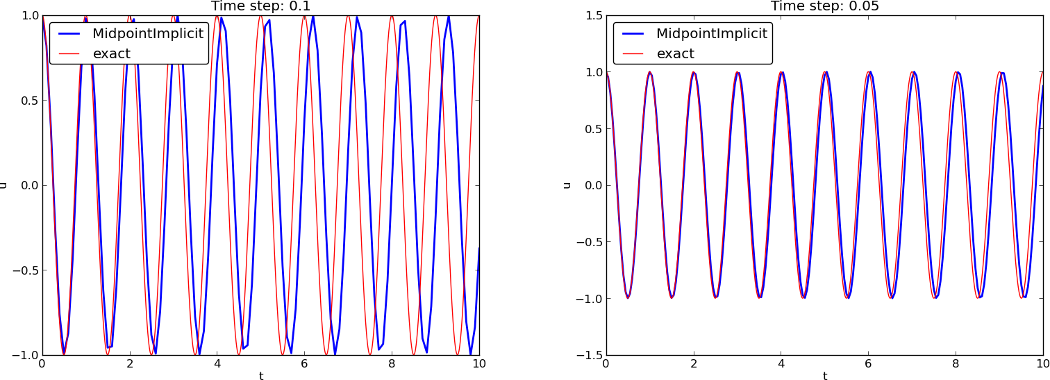
(MidpointImplicit means CrankNicolson in Odespy)

Observations of RK and CN methods

• 4th-order Runge-Kutta is very accurate, also for large \( \Delta t \).
• 2th-order Runge-Kutta is almost as bad as Forward and Backward Euler.
• Crank-Nicolson is accurate, but the amplitude is not as accurate as the difference scheme for \( u''+\omega^2u=0 \).

Energy conservation property

The model

$$ u'' + \omega^2 u = 0,\quad u(0)=I,\ u'(0)=V,$$ has the nice energy conservation property that

$$ E(t) = \half(u')^2 + \half\omega^2u^2 = \hbox{const}\tp$$ This can be used to check solutions.

Derivation of the energy conservation property

Multiply \( u''+\omega^2u=0 \) by \( u' \) and integrate:

$$ \int_0^T u''u' dt + \int_0^T\omega^2 u u' dt = 0\tp$$ Observing that

$$ u''u' = \frac{d}{dt}\half(u')^2,\quad uu' = \frac{d}{dt} {\half}u^2,$$ we get

$$ \int_0^T (\frac{d}{dt}\half(u')^2 + \frac{d}{dt} \half\omega^2u^2)dt = E(T) - E(0), $$ where

$$ \begin{equation} E(t) = \half(u')^2 + \half\omega^2u^2\tp \label{vib:model1:energy:balance1} \end{equation} $$

Remark about \( E(t) \)

\( E(t) \) does not measure energy, energy per mass unit.

Starting with an ODE coming directly from Newton's 2nd law \( F=ma \) with a spring force \( F=-ku \) and \( ma=mu'' \) (\( a \): acceleration, \( u \): displacement), we have

$$ mu'' + ku = 0$$ Integrating this equation gives a physical energy balance:

$$ E(t) = \underbrace{{\half}mv^2}_{\hbox{kinetic energy} } + \underbrace{{\half}ku^2}_{\hbox{potential energy}} = E(0),\quad v=u' $$ Note: the balance is not valid if we add other terms to the ODE.

The Euler-Cromer method; idea

Forward-backward discretization of the 2x2 system:

• Update \( u \) with Forward Euler
• Update \( v \) with Backward Euler, using latest \( u \)

$$ [D_t^-v = -\omega u]^{n+1} \tp $$

The Euler-Cromer method; complete formulas

Written out:

$$ \begin{align} u^0 &= I,\\ v^0 &= 0,\\ u^{n+1} &= u^n + \Delta t v^n, \label{vib:model2x2:EulerCromer:ueq1}\\ v^{n+1} &= v^n -\Delta t \omega^2u^{n+1} \label{vib:model2x2:EulerCromer:veq1} \tp \end{align} $$

Names: Forward-backward scheme, Semi-implicit Euler method, symplectic Euler, semi-explicit Euler, Newton-Stormer-Verlet, and Euler-Cromer.

• Forward Euler and Backward Euler have error \( \Oof{\Delta t} \)
• What about the overall scheme? Expect \( \Oof{\Delta t} \)...

Equivalence with the scheme for the second-order ODE

Goal: eliminate \( v^n \). We have $$ v^n = v^{n-1} - \Delta t \omega^2u^{n}, $$ which can be inserted in \eqref{vib:model2x2:EulerCromer:ueq1} to yield $$ \begin{equation} u^{n+1} = u^n + \Delta t v^{n-1} - \Delta t^2 \omega^2u^{n} . \label{vib:model2x2:EulerCromer:elim1} \end{equation} $$ Using \eqref{vib:model2x2:EulerCromer:ueq1}, $$ v^{n-1} = \frac{u^n - u^{n-1}}{\Delta t}, $$ and when this is inserted in \eqref{vib:model2x2:EulerCromer:elim1} we get $$ \begin{equation} u^{n+1} = 2u^n - u^{n-1} - \Delta t^2 \omega^2u^{n} \end{equation} $$

Comparison of the treatment of initial conditions

• The Euler-Cromer scheme is nothing but the centered scheme for \( u''+\omega^2u=0 \) \eqref{vib:model1:step4}!
• The previous analysis of this scheme then also applies to the Euler-Cromer method!
• What about the initial conditions?

This \( u^1=u^0 \) approximation corresponds to a first-order Forward Euler discretization of \( u'(0)=0 \): \( [D_t^+ u = 0]^0 \).

A method utilizing a staggered mesh

• The Euler-Cromer scheme uses two unsymmetric differences in a symmetric way...
• We can derive the method from a more pedagogical point of view where we use a staggered mesh and only centered differences

• \( u \) is unknown at mesh points \( t_0,t_1,\ldots,t_n,\ldots \)
• \( v \) is unknown at mesh points \( t_{1/2}, t_{3/2},\ldots, t_{n+1/2},\ldots \) (between the \( u \) points)

Centered differences on a staggered mesh

$$ \begin{align} \lbrack D_t u &= v\rbrack^{n+\half},\\ \lbrack D_t v &= -\omega u\rbrack^{n+1} \tp \end{align} $$ Written out:

$$ \begin{align} u^{n+1} &= u^{n} + \Delta t v^{n+\half}, \label{vib:model2x2:EulerCromer:ueq1s}\\ v^{n+\frac{3}{2}} &= v^{n+\half} -\Delta t \omega^2u^{n+1} \label{vib:model2x2:EulerCromer:veq1s} \tp \end{align} $$ or shift one time level back (purely of esthetic reasons):

$$ \begin{align} u^{n} &= u^{n-1} + \Delta t v^{n-\half}, \label{vib:model2x2:EulerCromer:ueq1s2}\\ v^{n+\half} &= v^{n-\half} -\Delta t \omega^2u^{n} \label{vib:model2x2:EulerCromer:veq1s2} \tp \end{align} $$

Comparison with the scheme for the 2nd-order ODE

• Can eliminate \( v^{n\pm 1/2} \) and get the centered scheme for \( u''+\omega^2 u = 0 \)
• What about the initial conditions? Their equivalent too!

$$ v(0)\approx \half(v^{-\half} + v^{\half}) = 0, \quad\Rightarrow\quad v^{-\half} =- v^\half\tp$$ Combined with the scheme on the staggered mesh we get

$$ u^1 = u^0 - \half\Delta t^2\omega^2 I,$$

Implementation of a staggered mesh; integer indices

• How to write \( v^{n+\half} \) in the code? v[i+0.5] does not work...
• Need a storage convention:

• \( v^{1+\half} \) $\rightarrow$ v[n]
• \( v^{1-\half} \) $\rightarrow$ v[n-1]
• \( v^{n+\half} = v^{n-\half} -\Delta t \omega^2u^{n} \) becomes v[n] = v[n-1] - dt*w**2*u[n]

!bc pycod
def solver(I, w, dt, T):
    # set up variables...

    u[0] = I
    v[0] = 0 - 0.5*dt*w**2*u[0]
    for n in range(1, Nt+1):
        u[n] = u[n-1] + dt*v[n-1]
        v[n] = v[n-1] - dt*w**2*u[n]
    return u, t, v, t_v

Implementation of a staggered mesh; half-integer indices (1)

It would be nice to write

$$ \begin{align*} u^{n} &= u^{n-1} + \Delta t v^{n-\half},\\ v^{n+\half} &= v^{n-\half} -\Delta t \omega^2u^{n}, \end{align*} $$ as

u[n] = u[n-1] + dt*v[n-half]
v[n+half] = v[n-half] - dt*w**2*u[n]

(Implying that n+half is n and n-half is n-1.)

Implementation of a staggered mesh; half-integer indices (2)

This class ensures that n+half is n and n-half is n-1:

class HalfInt:
    def __radd__(self, other):
        return other

    def __rsub__(self, other):
        return other - 1

half = HalfInt()

Now

u[n] = u[n-1] + dt*v[n-half]
v[n+half] = v[n-half] - dt*w**2*u[n]

is equivalent to

u[n] = u[n-1] + dt*v[n-1]
v[n] = v[n-1] - dt*w**2*u[n]

Generalization: damping, nonlinear spring, and external excitation

$$ \begin{equation} mu'' + f(u') + s(u) = F(t),\quad u(0)=I,\ u'(0)=V,\ t\in (0,T] \tp \label{vib:ode2} \end{equation} $$ Input data: \( m \), \( f(u') \), \( s(u) \), \( F(t) \), \( I \), \( V \), and \( T \).

Typical choices of \( f \) and \( s \):

• linear damping \( f(u')=bu \), or
• quadratic damping \( f(u')=bu'|u'| \)
• linear spring \( s(u)=cu \)
• nonlinear spring \( s(u)\sim \sin(u) \) (pendulum)

A centered scheme for linear damping

$$ \begin{equation} [mD_tD_t u + f(D_{2t}u) + s(u) = F]^n \end{equation} $$ Written out

$$ \begin{equation} m\frac{u^{n+1}-2u^n + u^{n-1}}{\Delta t^2} + f(\frac{u^{n+1}-u^{n-1}}{2\Delta t}) + s(u^n) = F^n \label{vib:ode2:step3b} \end{equation} $$ Assume \( f(u') \) is linear in \( u'=v \):

$$ \begin{equation} u^{n+1} = \left(2mu^n + (\frac{b}{2}\Delta t - m)u^{n-1} + \Delta t^2(F^n - s(u^n)) \right)(m + \frac{b}{2}\Delta t)^{-1} \label{vib:ode2:step4} \tp \end{equation} $$

Initial conditions

\( u(0)=I \), \( u'(0)=V \):

$$ \begin{align} \lbrack u &=I\rbrack^0\quad\Rightarrow\quad u^0=I,\\ \lbrack D_{2t}u &=V\rbrack^0\quad\Rightarrow\quad u^{-1} = u^{1} - 2\Delta t V \end{align} $$ End result:

$$ \begin{equation} u^1 = u^0 + \Delta t\, V + \frac{\Delta t^2}{2m}(-bV - s(u^0) + F^0) \tp \label{vib:ode2:step4b} \end{equation} $$ Same formula for \( u^1 \) as when using a centered scheme for \( u''+\omega u=0 \).

Linearization via a geometric mean approximation

• \( f(u')=bu'|u'| \) leads to a quadratic equation for \( u^{n+1} \)
• Instead of solving the quadratic equation, we use a geometric mean approximation

$$ [u'|u'|]^n \approx u'(t_n+{\half})|u'(t_n-{\half})|\tp$$ For \( u' \) at \( t_{n\pm 1/2} \) we use centered difference:

$$ \begin{equation} u'(t_{n+1/2})\approx [D_t u]^{n+\half},\quad u'(t_{n-1/2})\approx [D_t u]^{n-\half} \tp \label{vib:ode2:quad:idea2} \end{equation} $$

A centered scheme for quadratic damping

After some algebra:

$$ \begin{align} u^{n+1} &= \left( m + b|u^n-u^{n-1}|\right)^{-1}\times \nonumber\\ & \qquad \left(2m u^n - mu^{n-1} + bu^n|u^n-u^{n-1}| + \Delta t^2 (F^n - s(u^n)) \right) \tp \label{vib:ode2:step4:quad} \end{align} $$

Initial condition for quadratic damping

Simply use that \( u'=V \) in the scheme when \( t=0 \) (\( n=0 \)):

$$ \begin{equation} [mD_tD_t u + bV|V| + s(u) = F]^0 \end{equation} $$

which gives

$$ \begin{equation} u^1 = u^0 + \Delta t V + \frac{\Delta t^2}{2m}\left(-bV|V| - s(u^0) + F^0\right) \tp \label{vib:ode2:step4b:quad} \end{equation} $$

Algorithm

1. \( u^0=I \)
2. compute \( u^1 \) from \eqref{vib:ode2:step4b} if linear damping or \eqref{vib:ode2:step4b:quad} if quadratic damping
3. for \( n=1,2,\ldots,N_t-1 \):

1. compute \( u^{n+1} \) from \eqref{vib:ode2:step4} if linear damping or \eqref{vib:ode2:step4:quad} if quadratic damping

Implementation

def solver(I, V, m, b, s, F, dt, T, damping='linear'):
    dt = float(dt); b = float(b); m = float(m) # avoid integer div.
    Nt = int(round(T/dt))
    u = zeros(Nt+1)
    t = linspace(0, Nt*dt, Nt+1)

    u[0] = I
    if damping == 'linear':
        u[1] = u[0] + dt*V + dt**2/(2*m)*(-b*V - s(u[0]) + F(t[0]))
    elif damping == 'quadratic':
        u[1] = u[0] + dt*V + \ 
               dt**2/(2*m)*(-b*V*abs(V) - s(u[0]) + F(t[0]))

    for n in range(1, Nt):
        if damping == 'linear':
            u[n+1] = (2*m*u[n] + (b*dt/2 - m)*u[n-1] +
                      dt**2*(F(t[n]) - s(u[n])))/(m + b*dt/2)
        elif damping == 'quadratic':
            u[n+1] = (2*m*u[n] - m*u[n-1] + b*u[n]*abs(u[n] - u[n-1])
                      + dt**2*(F(t[n]) - s(u[n])))/\ 
                      (m + b*abs(u[n] - u[n-1]))
    return u, t

Verification

• Constant solution \( \uex = I \) (\( V=0 \)) fulfills the ODE problem and the discrete equations. Ideal for debugging!
• Linear solution \( \uex = Vt+I \) fulfills the ODE problem and the discrete equations.
• Quadratic solution \( \uex = bt^2 + Vt + I \) fulfills the ODE problem and the discrete equations with linear damping, but not for quadratic damping. A special discrete source term can allow \( \uex \) to also fulfill the discrete equations with quadratic damping.

Demo program

vib.py supports input via the command line:

Terminal> python vib.py --s 'sin(u)' --F '3*cos(4*t)' --c 0.03

This results in a moving window following the function on the screen.

Euler-Cromer formulation

We rewrite

$$ \begin{equation} mu'' + f(u') + s(u) = F(t),\quad u(0)=I,\ u'(0)=V,\ t\in (0,T], \end{equation} $$ as a first-order ODE system

$$ \begin{align} u' &= v, \label{vib:ode2:staggered:ueq} \\ v' &= m^{-1}\left(F(t) - f(v) - s(u)\right)\tp \label{vib:ode2:staggered:veq} \end{align} $$

Staggered grid

• \( u \) is unknown at \( t_n \): \( u^n \)
• \( v \) is unknown at \( t_{n+1/2} \): \( v^{n+\half} \)
• All derivatives are approximated by centered differences

Written out,

$$ \begin{align} \frac{u^n - u^{n-1}}{\Delta t} &= v^{n-\half}, \label{vib:ode2:staggered:dueq2} \\ \frac{v^{n+\half} - v^{n-\half}}{\Delta t} &= m^{-1}\left(F^n - f(v^n) - s(u^n)\right)\tp \label{vib:ode2:staggered:dveq2} \end{align} $$

Problem: \( f(v^n) \)

Linear damping

With \( f(v)=bv \), we can use an arithmetic mean for \( bv^n \) a la Crank-Nicolson schemes.

$$ \begin{align*} u^n & = u^{n-1} + {\Delta t}v^{n-\half},\\ v^{n+\half} &= \left(1 + \frac{b}{2m}\Delta t\right)^{-1}\left( v^{n-\half} + {\Delta t} m^{-1}\left(F^n - {\half}f(v^{n-\half}) - s(u^n)\right)\right)\tp \end{align*} $$

Quadratic damping

With \( f(v)=b|v|v \), we can use a geometric mean

$$ b|v^n|v^n\approx b|v^{n-\half}|v^{n+\half}, $$ resulting in

$$ \begin{align*} u^n & = u^{n-1} + {\Delta t}v^{n-\half},\\ v^{n+\half} &= (1 + \frac{b}{m}|v^{n-\half}|\Delta t)^{-1}\left( v^{n-\half} + {\Delta t} m^{-1}\left(F^n - s(u^n)\right)\right)\tp \end{align*} $$

Initial conditions

$$ \begin{align} u^0 &= I, \label{vib:ode2:staggered:u0}\\ v^{\half} &= V - \half\Delta t\omega^2I \label{vib:ode2:staggered:v0}\tp \end{align} $$