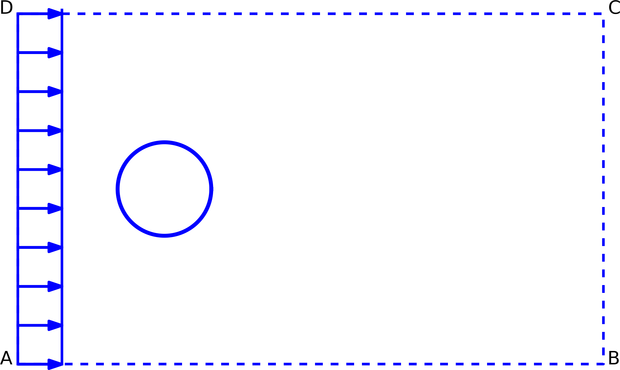
Figure 1: Flow around a cylinder.
The physical and mathematical problem
The Navier-Stokes equations
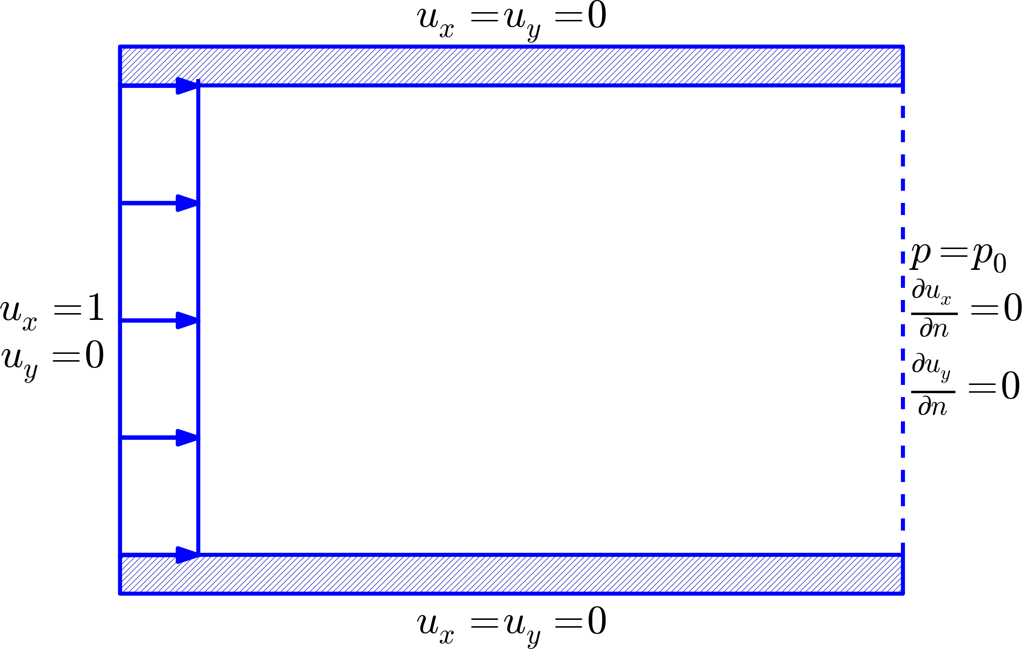
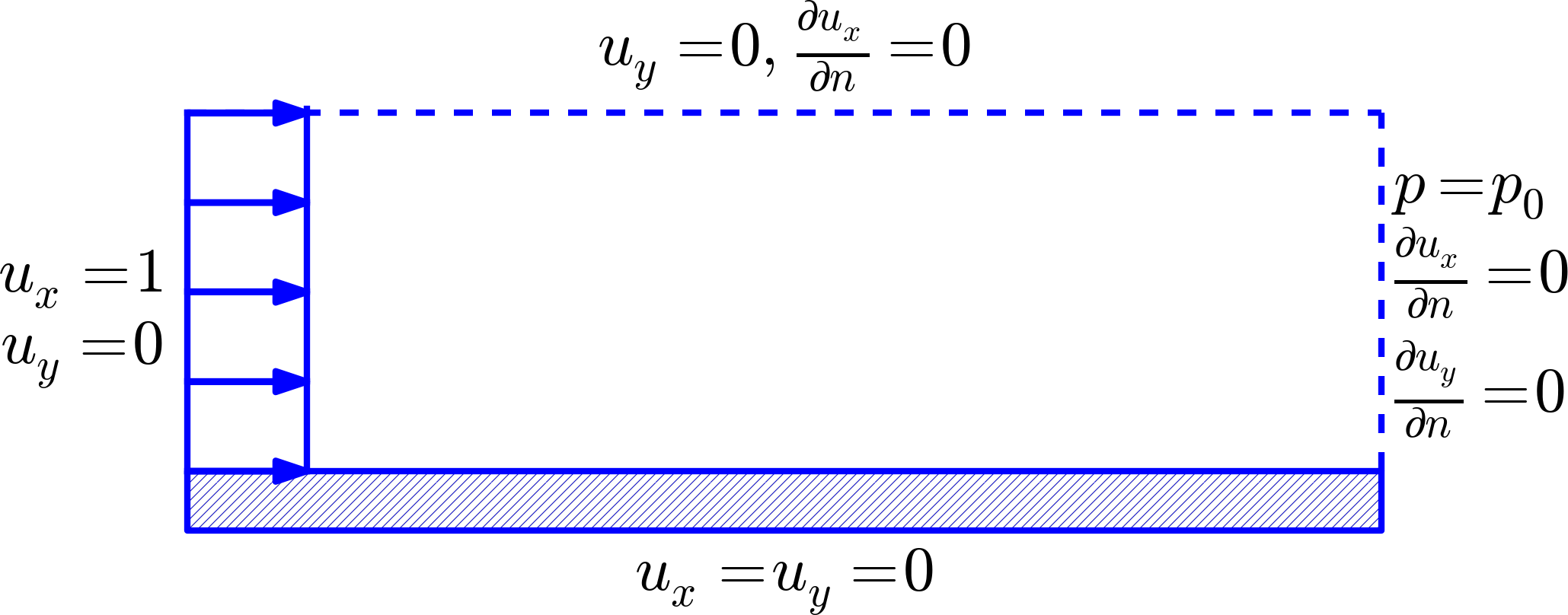
Boundary conditions
The classical splitting method
A simple, naive approach
A working scheme
Summary
Boundary conditions
Spatial discretization by the finite element method
Increasing the implicitness
Methods based on slight compressibility
Applications
Applications involving fluid flow:
Assumptions:
Figure 1: Flow around a cylinder.
Momentum balance (Newton's 2nd law):
uut+(uu⋅∇)uu=−1ϱ∇p+ν∇2uu+ff,
Mass balance (eq. of continuity):
∇⋅uu=0.
Idea: split the N-S equations into simpler problems (operator splitting).
The equation for uu looks like a diffusion equation...why not a Forward Euler scheme?
uut+(uu⋅∇)uu=−1ϱ∇p+ν∇2uu+ff
uun+1−uunΔt+(uun⋅∇)uun=−1ϱ∇pn+ν∇2uun+ffn,
uun+1=uun−Δt(uun⋅∇)uun−Δtϱ∇pn+Δtν∇2uun+Δtffn.
Two fundamental problems:
Idea: Forward Euler in time, but evaluate ∇p at tn+1 and enforce ∇⋅uun+1=0.
uun+1=uun−Δt(uun⋅∇)uun−Δtϱ∇pn+1+Δtν∇2uun+Δtffn,∇⋅uun+1=0
uu∗=uun−Δt(uun⋅∇)uun−βΔtϱ∇pn+Δtν∇2uun+Δtffn
Seek correction δuu such that
uun+1=uu∗+δuu, fulfills
∇⋅uun+1=0.
Subtract uu∗ equation from original uun+1 equation to find δuu:
δuu=uun+1−uu∗=−Δtϱ∇Φ, where
Φ=pn+1−βpn.
The oldest methods had β=0, but β≠0 gives in general better speed and accuracy.
∇⋅uun+1=0 implies
∇⋅δuu=−∇⋅uu∗, which gives
∇2Φ=ϱΔt∇⋅uu∗.
When Φ is computed,
uun+1=uu∗−Δtϱ∇Φ, and
pn+1=Φ+βpn.
Problem: p condition at one point only in the original N-S equations. Now we need boundary conditions for Φ along the whole boundary (Poisson equation).
Natural boundary condition:
ν∂uu∂n−pnn(=0) Usually ∂uu/∂n=0 and p=0 at outlets.
Pressure Poisson equation:
∫Ω∇Φ⋅∇v(Φ)dx=ϱΔt∫Ω∇⋅uu∗v(Φ)dx+∫∂ΩN,p∂Φ∂nv(Φ)ds,∀v(Φ)∈V(Φ).
Velocity update:
∫Ωuu⋅vv(u)dx=∫Ω(uu∗−Δtϱ∇Φ)⋅vv(u)dx,∀vv(u)∈V(u).
Pressure update:
∫Ωpv(Φ)dx=∫Ω(Φ+βp1)v(Φ)dx,∀v(Φ)∈V(Φ).
Stability (due to Forward Euler-style scheme):
Δt≤h22ν+Uh. h: minimum element size, U: typical velocity.
Better stability by a Backward Euler scheme:
uun+1=uun−Δt(uun+1⋅∇)uun+1−Δtϱ∇pn+1+Δtν∇2uun+1+Δtffn+1,∇⋅uun+1=0.
Intermediate velocity (∇pn+1→βpn):
uu∗=uun−Δt(uu∗⋅∇)uu∗−βΔtϱpn+1+Δtν∇2uu∗+Δtffn+1
Deal with nonlinearity in a simple way (1 Pickard it.):
(uu∗⋅∇)uu∗≈(uun⋅∇)uu∗.
Then we have a linear problem for uu∗:
uu∗=uun−Δt(uun⋅∇)uu∗−βΔtϱ∇pn+Δtν∇2uu∗+Δtffn+1
Correction (assume uun+1−uu∗ small):
δuu=Δt((uun+1⋅∇)uun+1−(uun⋅∇)uu∗)−Δtϱ∇Φ+Δtν(∇2(uun+1−uu∗)≈−Δtϱ∇Φ.
So, as before,
∇2Φ=ϱΔt∇⋅uu∗
∇⋅uu=0 is problematic. Allow slight compressibility in the fluid:
pt+c2∇⋅uu=0. c: speed of sound.
Now we have evolution equations for uu and p:
uut=−(uu⋅∇)uu−1ϱ∇p+ν∇2uu+ff,pt=−c2∇⋅uu.
Forward Euler:
uun+1=uun−Δt(uun⋅∇)uun−Δtϱ∇pn+Δtν∇2uun+Δtffn,pn+1=pn−Δtc2∇⋅uun.