
Why finite elements?
Domain for flow around a dolphin
The flow
Basic ingredients of the finite element method
Our learning strategy
Approximation in vector spaces
Approximation set-up
How to determine the coefficients?
Approximation of planar vectors; problem
Approximation of planar vectors; vector space terminology
The least squares method; principle
The least squares method; calculations
The projection (or Galerkin) method
Approximation of general vectors
The least squares method
The projection (or Galerkin) method
Approximation of functions
The least squares method
The projection (or Galerkin) method
Example: linear approximation; problem
Example: linear approximation; solution
Example: linear approximation; plot
Implementation of the least squares method; ideas
Implementation of the least squares method; symbolic code
Implementation of the least squares method; numerical code
Implementation of the least squares method; plotting
Implementation of the least squares method; application
Perfect approximation; parabola approximating parabola
Perfect approximation; the general result
Perfect approximation; proof of the general result
Finite-precision/numerical computations
Ill-conditioning (1)
Ill-conditioning (2)
Fourier series approximation; problem and code
Fourier series approximation; plot
Fourier series approximation; improvements
Fourier series approximation; final results
Orthogonal basis functions
The collocation or interpolation method; ideas and math
The collocation or interpolation method; implementation
The collocation or interpolation method; approximating a parabola by linear functions
Lagrange polynomials; motivation and ideas
Lagrange polynomials; formula and code
Lagrange polynomials; successful example
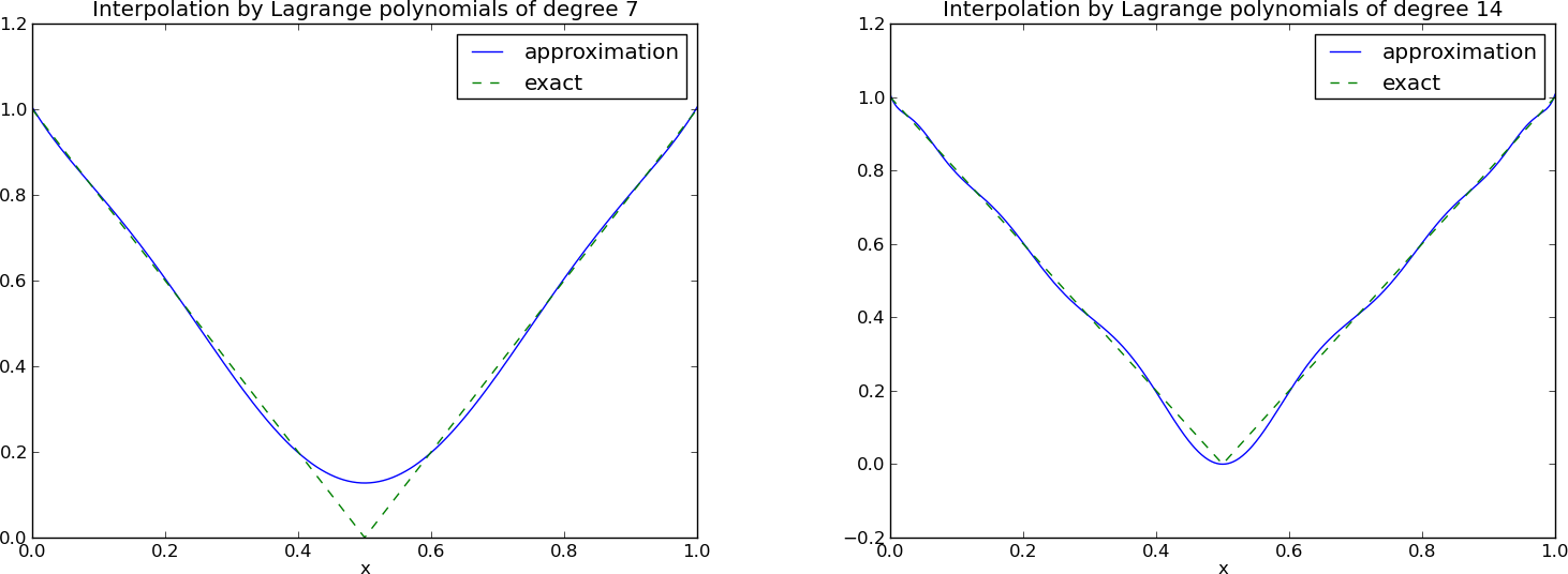
Lagrange polynomials; a less successful example
Lagrange polynomials; oscillatory behavior
Lagrange polynomials; remedy for strong oscillations
Lagrange polynomials; recalculation with Chebyshev nodes
Lagrange polynomials; less oscillations with Chebyshev nodes
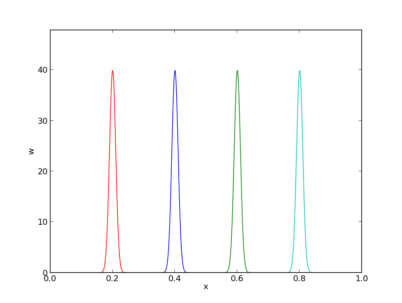
Finite element basis functions
The basis functions have so far been global: \( \baspsi_i(x) \neq 0 \) almost everywhere
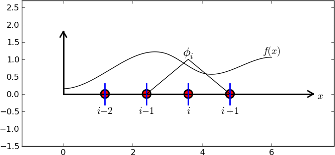
In the finite element method we use basis functions with local support
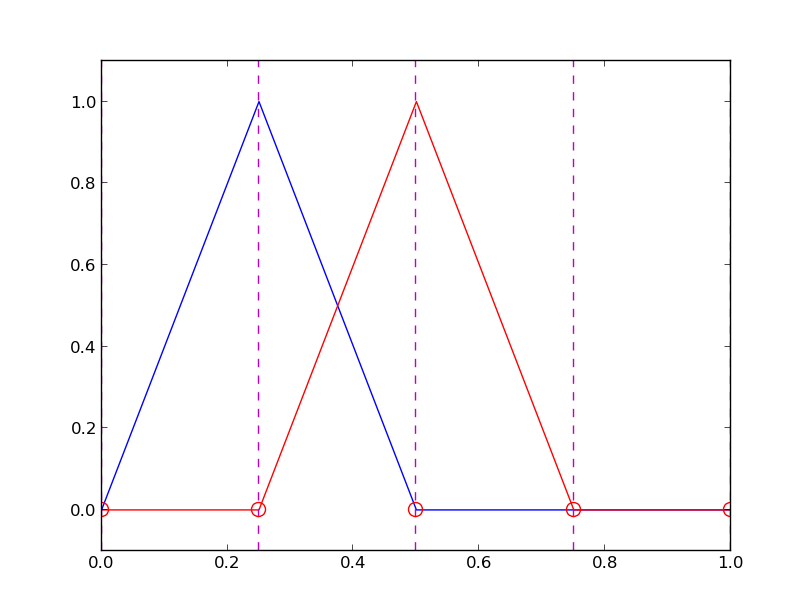
The linear combination of hat functions is a piecewise linear function
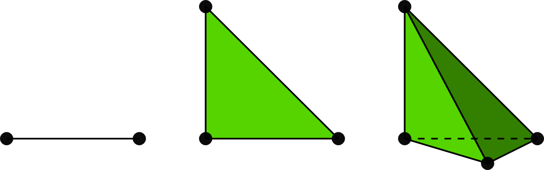
Elements and nodes
Example on elements with two nodes (P1 elements)
Illustration of two basis functions on the mesh
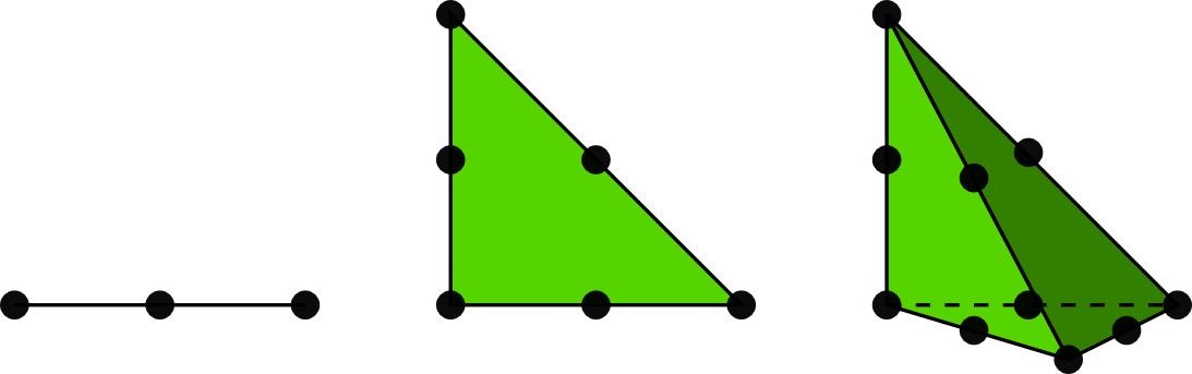
Example on elements with three nodes (P2 elements)
Some corresponding basis functions (P2 elements)
Examples on elements with four nodes per element (P3 elements)
Some corresponding basis functions (P3 elements)
The numbering does not need to be regular from left to right
Interpretation of the coefficients \( c_i \)
Properties of the basis functions
How to construct quadratic \( \basphi_i \) (P2 elements)
Example on linear \( \basphi_i \) (P1 elements)
Example on cubic \( \basphi_i \) (P3 elements)
Calculating the linear system for \( c_i \)
Computing a specific matrix entry (1)
Computing a specific matrix entry (2)
Calculating a general row in the matrix; figure
Calculating a general row in the matrix; details
Calculation of the right-hand side
Specific example with two elements; linear system and solution
Specific example with two elements; plot
Specific example: what about four elements?
Assembly of elementwise computations
Split the integrals into elementwise integrals
The element matrix
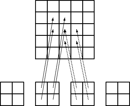
Illustration of the matrix assembly: regularly numbered P1 elements
Illustration of the matrix assembly: regularly numbered P3 elements
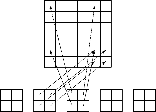
Illustration of the matrix assembly: irregularly numbered P1 elements
Assembly of the right-hand side
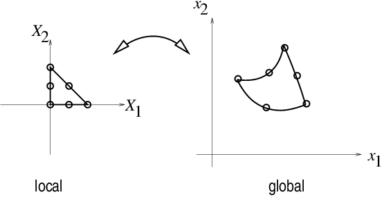
Mapping to a reference element
Affine mapping
Integral transformation
Advantages of the reference element
Standardized basis functions for P1 elements
Standardized basis functions for P2 elements
Integration over a reference element; element matrix
Integration over a reference element; element vector
Tedious calculations! Let's use symbolic software
Implementation
Compute finite element basis functions in the reference element
Compute the element matrix
Example on symbolic vs numeric element matrix
Compute the element vector
Fallback on numerical integration if symbolic integration fails
Linear system assembly and solution
Linear system solution
Example on computing symbolic approximations
Example on computing numerical approximations
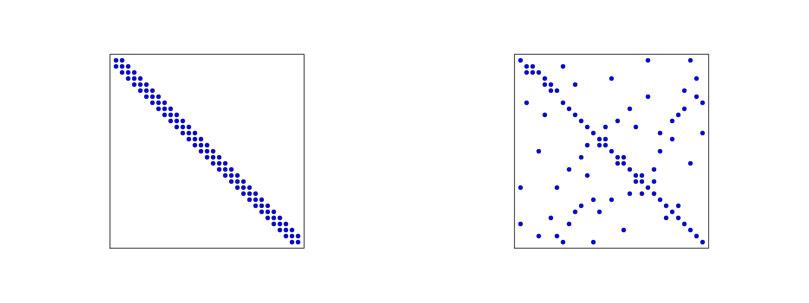
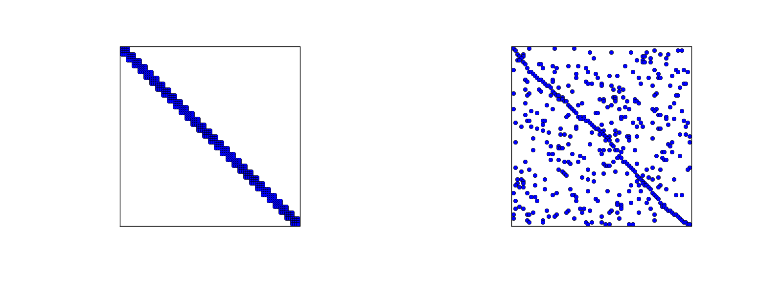
The structure of the coefficient matrix
General result: the coefficient matrix is sparse
Exemplifying the sparsity for P2 elements
Matrix sparsity pattern for regular/random numbering of P1 elements
Matrix sparsity pattern for regular/random numbering of P3 elements
Sparse matrix storage and solution
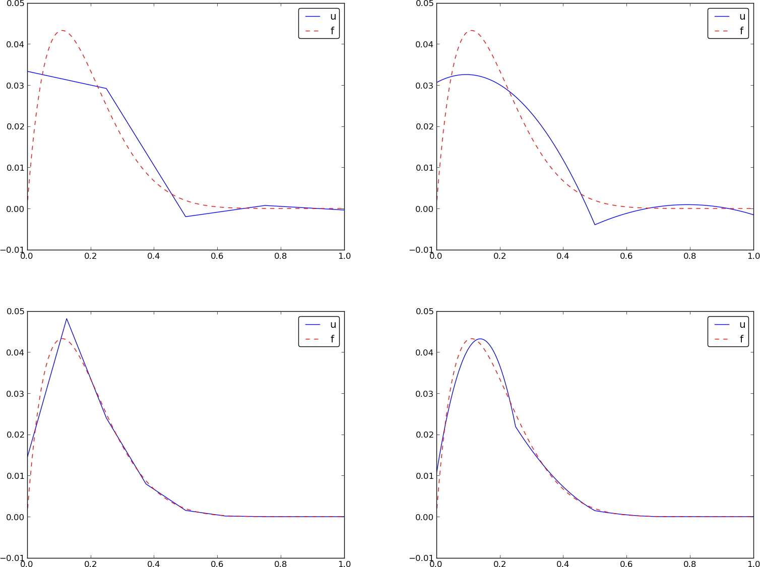
Approximate \( f\sim x^9 \) by various elements; code
Approximate \( f\sim x^9 \) by various elements; plot
Comparison of finite element and finite difference approximation
Interpolation/collocation with finite elements
Galerkin/project and least squares vs collocation/interpolation or finite differences
Expressing the left-hand side in finite difference operator notation
Treating the right-hand side; Trapezoidal rule
Treating the right-hand side; Simpson's rule
Finite element approximation vs finite differences
Making finite elements behave as finite differences
Limitations of the nodes and element concepts
A generalized element concept
The concept of a finite element
Implementation; basic data structures
Implementation; example with P2 elements
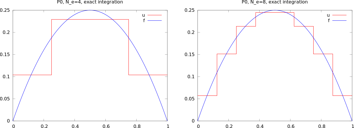
Implementation; example with P0 elements
Example on doing the algorithmic steps
Approximating a parabola by P0 elements
Computing the error of the approximation; principles
Computing the error of the approximation; details
How does the error depend on \( h \) and \( d \)?
Cubic Hermite polynomials; definition
Cubic Hermite polynomials; derivation
Cubic Hermite polynomials; result
Numerical integration
The Midpoint rule
Newton-Cotes rules
Gauss-Legendre rules with optimized points
Approximation of functions in 2D
2D basis functions as tensor products of 1D functions
Tensor products
Double or single index?
Example on 2D (bilinear) basis functions; formulas
Example on 2D (bilinear) basis functions; plot
Implementation; principal changes to the 1D code
Implementation; 2D integration
Implementation; 2D basis functions
Implementation; application
Implementation; trying a perfect expansion
Generalization to 3D
Finite elements in 2D and 3D
Examples on cell types
Rectangular domain with 2D P1 elements
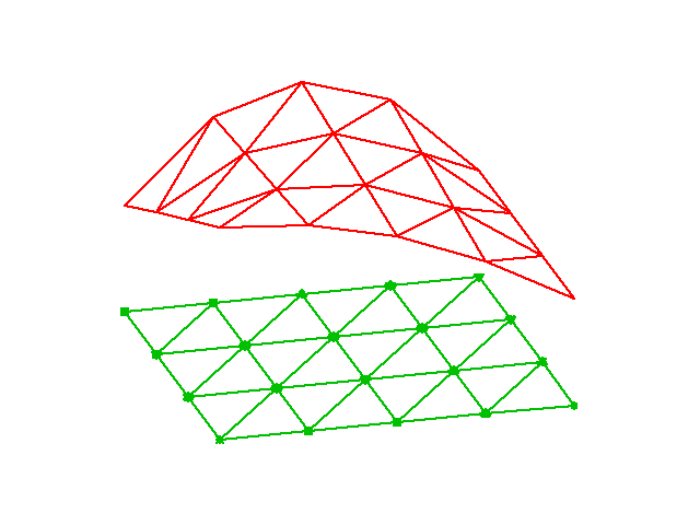
Deformed geometry with 2D P1 elements
Rectangular domain with 2D Q1 elements
Basis functions over triangles in the physical domain
Basic features of 2D P1 elements
Linear mapping of reference element onto general triangular cell
\( \basphi_i \): pyramid shape, composed of planes
Element matrices and vectors
Basis functions over triangles in the reference cell
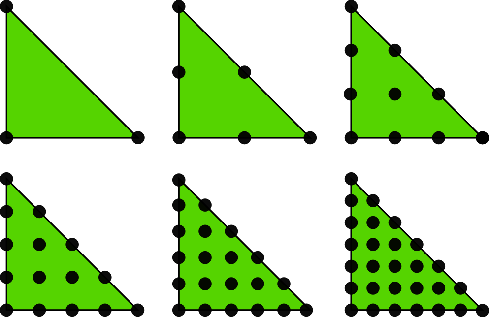
2D P1, P2, P3, P4, P5, and P6 elements
P1 elements in 1D, 2D, and 3D
P2 elements in 1D, 2D, and 3D
Affine mapping of the reference cell; formula
Affine mapping of the reference cell; figure
Isoparametric mapping of the reference cell
Computing integrals
Remark on going from 1D to 2D/3D
Differential equation models
Abstract differential equation
Abstract boundary conditions
Reminder about notation
New topics
Residual-minimizing principles
The least squares method
The Galerkin method
The Method of Weighted Residuals
Terminology: test and trial Functions
The collocation method
Examples on using the principles
The first model problem
Boundary conditions
The least squares method; principle
The least squares method; equation system
Orthogonality of the basis functions gives diagonal matrix
Least squares method; solution
The Galerkin method; principle
The Galerkin method; solution
The collocation method
Comparison of the methods
Useful techniques
Integration by parts
Boundary function; principles
Boundary function; example (1)
Boundary function; example (2)
Impact of the boundary function on the space where we seek the solution
Abstract notation for variational formulations
Example on abstract notation
Bilinear and linear forms
The linear system associated with abstract form
Equivalence with minimization problem
Examples on variational formulations
Variable coefficient; problem
Variable coefficient; variational formulation (1)
Variable coefficient; variational formulation (2)
Variable coefficient; linear system (the easy way)
Variable coefficient; linear system (full derivation)
First-order derivative in the equation and boundary condition; problem
First-order derivative in the equation and boundary condition; details
First-order derivative in the equation and boundary condition; observations
First-order derivative in the equation and boundary condition; abstract notation
First-order derivative in the equation and boundary condition; linear system
Terminology: natural and essential boundary conditions
Nonlinear coefficient; problem
Nonlinear coefficient; variational formulation
Nonlinear coefficient; where does the nonlinearity cause challenges?
Computing with Dirichlet and Neumann conditions; problem
Computing with Dirichlet and Neumann conditions; details
When the numerical method is exact
Computing with finite elements
Variational formulation, finite element mesh, and basis
Computation in the global physical domain; formulas
Computation in the global physical domain; details
Computation in the global physical domain; linear system
Comparison with a finite difference discretization
Cellwise computations; formulas
Cellwise computations; details
Cellwise computations; details of boundary cells
Cellwise computations; assembly
General construction of a boundary function
Example with two Dirichlet values; variational formulation
Example with two Dirichlet values; boundary function
Example with two Dirichlet values; details
Example with two Dirichlet values; cellwise computations
Modification of the linear system; ideas
Modification of the linear system; original system
Modification of the linear system; row replacement
Modification of the linear system; element matrix/vector
Symmetric modification of the linear system; algorithm
Symmetric modification of the linear system; example
Symmetric modification of the linear system; element level
Boundary conditions: specified derivative
The variational formulation
Method 1: Boundary function and exclusion of Dirichlet degrees of freedom
Method 2: Use all \( \basphi_i \) and insert the Dirichlet condition in the linear system
How the Neumann condition impacts the element matrix and vector
The finite element algorithm
Python pseudo code; the element matrix and vector
Python pseudo code; boundary conditions and assembly
Variational formulations in 2D and 3D
Integration by parts
Example on integration by parts; problem
Example on integration by parts; details (1)
Example on integration by parts; details (2)
Example on integration by parts; linear system
Transformation to a reference cell in 2D/3D (1)
Transformation to a reference cell in 2D/3D (2)
Numerical integration
Time-dependent problems
Example: diffusion problem
A Forward Euler scheme; ideas
A Forward Euler scheme; stages in the discretization
A Forward Euler scheme; weighted residual (or Galerkin) principle
A Forward Euler scheme; integration by parts
New notation for the solution at the most recent time levels
Deriving the linear systems
Structure of the linear systems
Computational algorithm
Comparing P1 elements with the finite difference method; ideas
Comparing P1 elements with the finite difference method; results
Discretization in time by a Backward Euler scheme
The variational form of the time-discrete problem
Calculations with P1 elements in 1D
Dirichlet boundary conditions
Boundary function
Finite element basis functions
Modification of the linear system; the raw system
Modification of the linear system; setting Dirichlet conditions
Modification of the linear system; Backward Euler example
Analysis of the discrete equations
Handy formulas
Amplification factor for the Forward Euler method; results
Amplification factor for the Backward Euler method; results
Amplification factors for smaller time steps; Forward Euler
Amplification factors for smaller time steps; Backward Euler

General idea of finding an approximation \( u(x) \) to some given \( f(x) \):
$$ \begin{equation} u(x) = \sum_{i=0}^N c_i\baspsi_i(x) \label{fem:u} \end{equation} $$
where
We shall address three approaches:
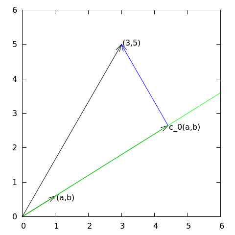
Given a vector \( \f = (3,5) \), find an approximation to \( \f \) directed along a given line.
$$ \begin{equation} V = \mbox{span}\,\{ \psib_0\} \end{equation} $$
$$ \begin{equation} E(c_0) = (\e,\e) = (\f,\f) - 2c_0(\f,\psib_0) + c_0^2(\psib_0,\psib_0) \end{equation} $$
$$ \begin{equation} \frac{\partial E}{\partial c_0} = -2(\f,\psib_0) + 2c_0 (\psib_0,\psib_0) = 0 \label{fem:vec:dEdc0:v1} \end{equation} $$
$$ \begin{equation} c_0 = \frac{(\f,\psib_0)}{(\psib_0,\psib_0)} \label{fem:vec:c0} \end{equation} $$
$$ \begin{equation} c_0 = \frac{3a + 5b}{a^2 + b^2} \end{equation} $$
Observation for later: the vanishing derivative \eqref{fem:vec:dEdc0:v1} can be alternatively written as
$$ \begin{equation} (\e, \psib_0) = 0 \label{fem:vec:dEdc0:Galerkin} \end{equation} $$
Given a vector \( \f \), find an approximation \( \u\in V \):
$$ \begin{equation*} V = \hbox{span}\,\{\psib_0,\ldots,\psib_N\} \end{equation*} $$
Idea: find \( c_0,\ldots,c_N \) such that \( E= ||\e||^2 \) is minimized, \( \e=\f-\u \).
$$ \begin{align*} E(c_0,\ldots,c_N) &= (\e,\e) = (\f -\sum_jc_j\psib_j,\f -\sum_jc_j\psib_j) \nonumber\\ &= (\f,\f) - 2\sum_{j=0}^Nc_j(\f,\psib_j) + \sum_{p=0}^N\sum_{q=0}^N c_pc_q(\psib_p,\psib_q) \end{align*} $$
$$ \begin{equation*} \frac{\partial E}{\partial c_i} = 0,\quad i=0,\ldots,N \end{equation*} $$
After some work we end up with a linear system
$$ \begin{align} \sum_{j=0}^N A_{i,j}c_j &= b_i,\quad i=0,\ldots,N\\ A_{i,j} &= (\psib_i,\psib_j)\\ b_i &= (\psib_i, \f) \end{align} $$
Can be shown that minimizing \( ||\e|| \) implies that \( \e \) is orthogonal to all \( \v\in V \):
$$ (\e,\v)=0,\quad \forall\v\in V $$ which implies that \( \e \) most be orthogonal to each basis vector:
$$ \begin{equation} (\e,\psib_i)=0,\quad i=0,\ldots,N \label{fem:approx:vec:Np1dim:Galerkin0} \end{equation} $$
This orthogonality condition is the principle of the projection (or Galerkin) method. Leads to the same linear system as in the least squares method.
Let \( V \) be a function space spanned by a set of basis functions \( \baspsi_0,\ldots,\baspsi_N \),
$$ \begin{equation*} V = \hbox{span}\,\{\baspsi_0,\ldots,\baspsi_N\} \end{equation*} $$
Find \( u\in V \) as a linear combination of the basis functions:
$$ \begin{equation} u = \sum_{j\in\If} c_j\baspsi_j,\quad\If = \{0,1,\ldots,N\} \label{fem:approx:ufem} \end{equation} $$
$$ \begin{equation} E(c_0,\ldots,c_N) = (f,f) -2\sum_{j\in\If} c_j(f,\baspsi_i) + \sum_{p\in\If}\sum_{q\in\If} c_pc_q(\baspsi_p,\baspsi_q) \end{equation} $$
$$ \begin{equation*} \frac{\partial E}{\partial c_i} = 0,\quad i=\in\If \end{equation*} $$
After computations identical to the vector case, we get a linear system
$$ \begin{align} \sum_{j\in\If}^N A_{i,j}c_j &= b_i,\quad i\in\If \label{fem:approx:vec:Np1dim:eqsys}\\ A_{i,j} &= (\baspsi_i,\baspsi_j) \label{fem:approx:Aij}\\ b_i &= (f,\baspsi_i) \label{fem:approx:bi} \end{align} $$
As before, minimizing \( (e,e) \) is equivalent to the projection (or Galerkin) method
$$ \begin{equation} (e,v)=0,\quad\forall v\in V \label{fem:approx:Galerkin} \end{equation} $$ which means, as before,
$$ \begin{equation} (e,\baspsi_i)=0,\quad i\in\If \label{fem:approx:Galerkin0} \end{equation} $$
With the same algebra as in the multi-dimensional vector case, we get the same linear system as arose from the least squares method.
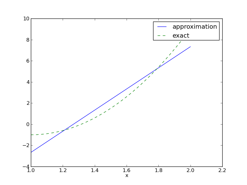
$$ \begin{equation*} V = \hbox{span}\,\{1, x\} \end{equation*} $$ That is, \( \baspsi_0(x)=1 \), \( \baspsi_1(x)=x \), and \( N=1 \). We seek
$$ \begin{equation*} u=c_0\baspsi_0(x) + c_1\baspsi_1(x) = c_0 + c_1x \end{equation*} $$
$$ \begin{align} A_{0,0} &= (\baspsi_0,\baspsi_0) = \int_1^21\cdot 1\, dx = 1\\ A_{0,1} &= (\baspsi_0,\baspsi_1) = \int_1^2 1\cdot x\, dx = 3/2\\ A_{1,0} &= A_{0,1} = 3/2\\ A_{1,1} &= (\baspsi_1,\baspsi_1) = \int_1^2 x\cdot x\,dx = 7/3 \end{align} $$
$$ \begin{align} b_1 &= (f,\baspsi_0) = \int_1^2 (10(x-1)^2 - 1)\cdot 1 \, dx = 7/3\\ b_2 &= (f,\baspsi_1) = \int_1^2 (10(x-1)^2 - 1)\cdot x\, dx = 13/3 \end{align} $$ Solution of 2x2 linear system:
$$ \begin{equation} c_0 = -38/3,\quad c_1 = 10,\quad u(x) = 10x - \frac{38}{3} \end{equation} $$
Consider symbolic computation of the linear system, where
sympy expression f (involving
the symbol x),psi is a list of \( \sequencei{\baspsi} \),Omega is a 2-tuple/list holding the domain \( \Omega \)
import sympy as sp

def least_squares(f, psi, Omega):
    N = len(psi) - 1
    A = sp.zeros((N+1, N+1))
    b = sp.zeros((N+1, 1))
    x = sp.Symbol('x')
    for i in range(N+1):
        for j in range(i, N+1):
            A[i,j] = sp.integrate(psi[i]*psi[j],
                                  (x, Omega[0], Omega[1]))
            A[j,i] = A[i,j]
        b[i,0] = sp.integrate(psi[i]*f, (x, Omega[0], Omega[1]))
    c = A.LUsolve(b)
    u = 0
    for i in range(len(psi)):
        u += c[i,0]*psi[i]
    return u, c
Observe: symmetric coefficient matrix so we can halve the integrations.
f(x), psi(x,i), and a mesh x
def least_squares_numerical(f, psi, N, x,
                            integration_method='scipy',
                            orthogonal_basis=False):
    import scipy.integrate
    A = np.zeros((N+1, N+1))
    b = np.zeros(N+1)
    Omega = [x[0], x[-1]]
    dx = x[1] - x[0]

    for i in range(N+1):
        j_limit = i+1 if orthogonal_basis else N+1
        for j in range(i, j_limit):
            print '(%d,%d)' % (i, j)
            if integration_method == 'scipy':
                A_ij = scipy.integrate.quad(
                    lambda x: psi(x,i)*psi(x,j),
                    Omega[0], Omega[1], epsabs=1E-9, epsrel=1E-9)[0]
            elif ...
            A[i,j] = A[j,i] = A_ij

        if integration_method == 'scipy':
            b_i = scipy.integrate.quad(
                lambda x: f(x)*psi(x,i), Omega[0], Omega[1],
                epsabs=1E-9, epsrel=1E-9)[0]
        elif ...
        b[i] = b_i

    c = b/np.diag(A) if orthogonal_basis else np.linalg.solve(A, b)
    u = sum(c[i]*psi(x, i) for i in range(N+1))
    return u, c
Compare \( f \) and \( u \) visually:
def comparison_plot(f, u, Omega, filename='tmp.pdf'):
    x = sp.Symbol('x')
    # Turn f and u to ordinary Python functions
    f = sp.lambdify([x], f, modules="numpy")
    u = sp.lambdify([x], u, modules="numpy")
    resolution = 401  # no of points in plot
    xcoor  = linspace(Omega[0], Omega[1], resolution)
    exact  = f(xcoor)
    approx = u(xcoor)
    plot(xcoor, approx)
    hold('on')
    plot(xcoor, exact)
    legend(['approximation', 'exact'])
    savefig(filename)
All code in module approx1D.py
>>> from approx1D import *
>>> x = sp.Symbol('x')
>>> f = 10*(x-1)**2-1
>>> u, c = least_squares(f=f, psi=[1, x], Omega=[1, 2])
>>> comparison_plot(f, u, Omega=[1, 2])
>>> from approx1D import *
>>> x = sp.Symbol('x')
>>> f = 10*(x-1)**2-1
>>> u, c = least_squares(f=f, psi=[1, x, x**2], Omega=[1, 2])
>>> print u
10*x**2 - 20*x + 9
>>> print sp.expand(f)
10*x**2 - 20*x + 9
least_squares is \( c_i=0 \) for \( i>2 \)
If \( f\in V \), \( f=\sum_{j\in\If}d_j\baspsi_j \), for some \( \sequencei{d} \). Then
$$ \begin{equation*} b_i = (f,\baspsi_i) = \sum_{j\in\If}d_j(\baspsi_j, \baspsi_i) = \sum_{j\in\If} d_jA_{i,j} \end{equation*} $$ The linear system \( \sum_j A_{i,j}c_j = b_i \), \( i\in\If \), is then
$$ \begin{equation*} \sum_{j\in\If}c_jA_{i,j} = \sum_{j\in\If}d_jA_{i,j},\quad i\in\If \end{equation*} $$ which implies that \( c_i=d_i \) for \( i\in\If \) and \( u \) is identical to \( f \).
The previous computations were symbolic. What if we solve the linear system numerically with standard arrays?
| exact | sympy | numpy32 | numpy64 |
| 9 | 9.62 | 5.57 | 8.98 |
| -20 | -23.39 | -7.65 | -19.93 |
| 10 | 17.74 | -4.50 | 9.96 |
| 0 | -9.19 | 4.13 | -0.26 |
| 0 | 5.25 | 2.99 | 0.72 |
| 0 | 0.18 | -1.21 | -0.93 |
| 0 | -2.48 | -0.41 | 0.73 |
| 0 | 1.81 | -0.013 | -0.36 |
| 0 | -0.66 | 0.08 | 0.11 |
| 0 | 0.12 | 0.04 | -0.02 |
| 0 | -0.001 | -0.02 | 0.002 |
sympy.mpmath.fp.matrix and sympy.mpmath.fp.lu_solvenumpy arrays with numpy.float32 entriesnumpy arrays with numpy.float64 entriesObservations:
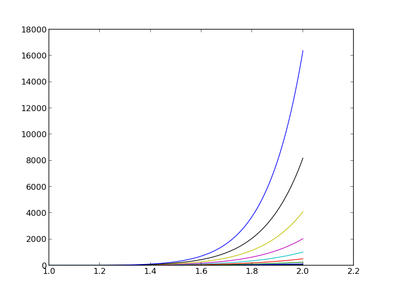
Consider
$$ \begin{equation*} V = \hbox{span}\,\{ \sin \pi x, \sin 2\pi x,\ldots,\sin (N+1)\pi x\} \end{equation*} $$
N = 3
from sympy import sin, pi
psi = [sin(pi*(i+1)*x) for i in range(N+1)]
f = 10*(x-1)**2 - 1
Omega = [0, 1]
u, c = least_squares(f, psi, Omega)
comparison_plot(f, u, Omega)
\( N=3 \) vs \( N=11 \):

\( N=3 \) vs \( N=11 \):

This choice of sine functions as basis functions is popular because
$$ c_i = \frac{b_i}{A_{i,i}} = \frac{(f,\baspsi_i)}{(\baspsi_i,\baspsi_i)} $$
Here is another idea for approximating \( f(x) \) by \( u(x)=\sum_jc_j\baspsi_j \):
This is a linear system with no need for integration:
$$ \begin{align} \sum_{j\in\If} A_{i,j}c_j &= b_i,\quad i\in\If\\ A_{i,j} &= \baspsi_j(\xno{i})\\ b_i &= f(\xno{i}) \end{align} $$
No symmetric matrix: \( \baspsi_j(\xno{i})\neq \baspsi_i(\xno{j}) \) in general
points holds the interpolation/collocation points
def interpolation(f, psi, points):
    N = len(psi) - 1
    A = sp.zeros((N+1, N+1))
    b = sp.zeros((N+1, 1))
    x = sp.Symbol('x')
    # Turn psi and f into Python functions
    psi = [sp.lambdify([x], psi[i]) for i in range(N+1)]
    f = sp.lambdify([x], f)
    for i in range(N+1):
        for j in range(N+1):
            A[i,j] = psi[j](points[i])
        b[i,0] = f(points[i])
    c = A.LUsolve(b)
    u = 0
    for i in range(len(psi)):
        u += c[i,0]*psi[i](x)
    return u

Motivation:
$$ \baspsi_i(\xno{j}) =\delta_{ij},\quad \delta_{ij} = \left\lbrace\begin{array}{ll} 1, & i=j\\ 0, & i\neq j \end{array}\right. $$
Hence, \( c_i = f(x_i) \) and
$$ \begin{equation} u(x) = \sum_{j\in\If} f(\xno{i})\baspsi_i(x) \end{equation} $$
$$ \begin{equation} \baspsi_i(x) = \prod_{j=0,j\neq i}^N \frac{x-\xno{j}}{\xno{i}-\xno{j}} = \frac{x-x_0}{\xno{i}-x_0}\cdots\frac{x-\xno{i-1}}{\xno{i}-\xno{i-1}}\frac{x-\xno{i+1}}{\xno{i}-\xno{i+1}} \cdots\frac{x-x_N}{\xno{i}-x_N} \label{fem:approx:global:Lagrange:poly} \end{equation} $$
def Lagrange_polynomial(x, i, points):
    p = 1
    for k in range(len(points)):
        if k != i:
            p *= (x - points[k])/(points[i] - points[k])
    return p
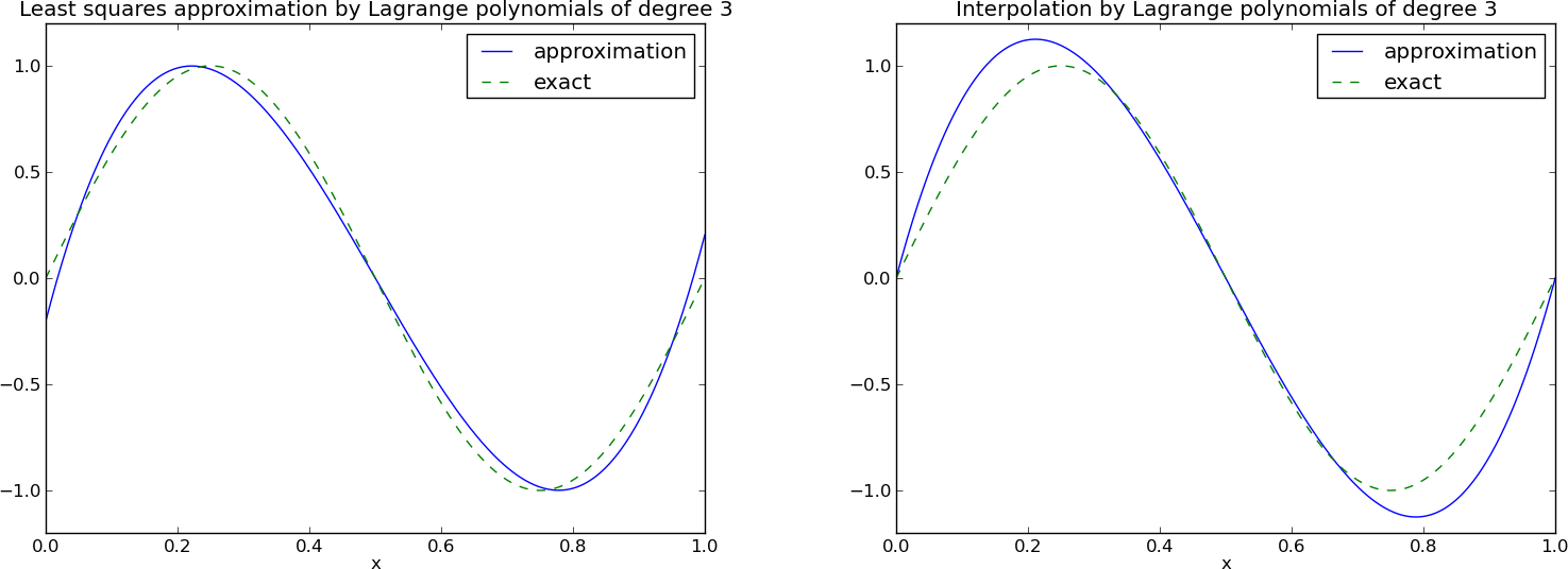

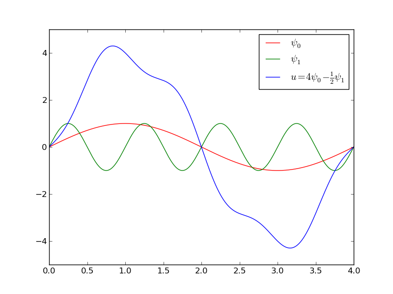
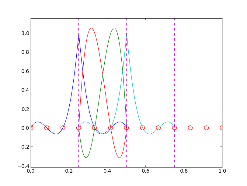
12 points, degree 11, plot of two of the Lagrange polynomials - note that they are zero at all points except one.

Problem: strong oscillations near the boundaries for larger \( N \) values.
The oscillations can be reduced by a more clever choice of interpolation points, called the Chebyshev nodes:
$$ \begin{equation} \xno{i} = \half (a+b) + \half(b-a)\cos\left( \frac{2i+1}{2(N+1)}pi\right),\quad i=0\ldots,N \end{equation} $$ on an interval \( [a,b] \).
12 points, degree 11, plot of two of the Lagrange polynomials - note that they are zero at all points except one.


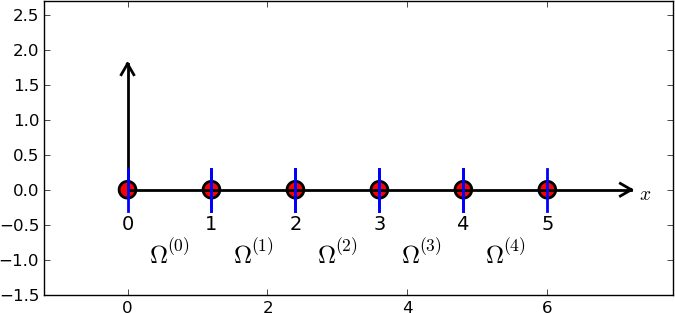
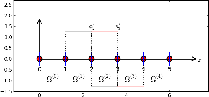
Split \( \Omega \) into non-overlapping subdomains called elements:
$$ \begin{equation} \Omega = \Omega^{(0)}\cup \cdots \cup \Omega^{(N_e)} \end{equation} $$
On each element, introduce points called nodes: \( \xno{0},\ldots,\xno{N_n} \)
Data structure: nodes holds coordinates or nodes, elements holds the
node numbers in each element
nodes = [0, 1.2, 2.4, 3.6, 4.8, 5]
elements = [[0, 1], [1, 2], [2, 3], [3, 4], [4, 5]]
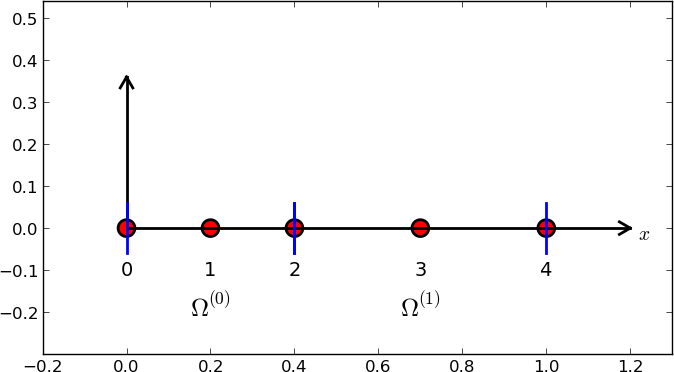
nodes = [0, 0.125, 0.25, 0.375, 0.5, 0.625, 0.75, 0.875, 1.0]
elements = [[0, 1, 2], [2, 3, 4], [4, 5, 6], [6, 7, 8]]


d = 3  # d+1 nodes per element
num_elements = 4
num_nodes = num_elements*d + 1
nodes = [i*0.5 for i in range(num_nodes)]
elements = [[i*d+j for j in range(d+1)] for i in range(num_elements)]
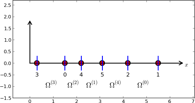
nodes = [1.5, 5.5, 4.2, 0.3, 2.2, 3.1]
elements = [[2, 1], [4, 5], [0, 4], [3, 0], [5, 2]]
Important property: \( c_i \) is the value of \( u \) at node \( i \), \( \xno{i} \):
$$ \begin{equation} u(\xno{i}) = \sum_{j\in\If} c_j\basphi_j(\xno{i}) = c_i\basphi_i(\xno{i}) = c_i \label{fem:approx:fe:phi:prop1} \end{equation} $$
because \( \basphi_j(\xno{i}) =0 \) if \( i\neq j \)
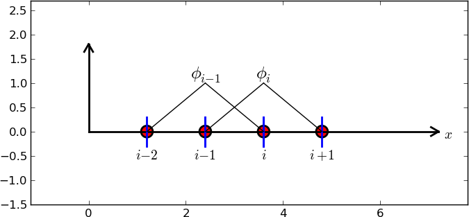
$$ \begin{equation} \basphi_i(x) = \left\lbrace\begin{array}{ll} 0, & x < \xno{i-1}\\ (x - \xno{i-1})/h & \xno{i-1} \leq x < \xno{i}\\ 1 - (x - x_{i})/h, & \xno{i} \leq x < \xno{i+1}\\ 0, & x\geq \xno{i+1} \end{array} \right. \label{fem:approx:fe:phi:1:formula2} \end{equation} $$
\( A_{2,3}=\int_\Omega\basphi_2\basphi_3 dx \): \( \basphi_2\basphi_3\neq 0 \) only over element 2. There,
$$ \basphi_3(x) = (x-x_2)/h,\quad \basphi_2(x) = 1- (x-x_2)/h$$
$$ A_{2,3} = \int_\Omega \basphi_2\basphi_{3}\dx = \int_{\xno{2}}^{\xno{3}} \left(1 - \frac{x - \xno{2}}{h}\right) \frac{x - x_{2}}{h} \dx = \frac{h}{6} $$
$$ A_{2,2} = \int_{\xno{1}}^{\xno{2}} \left(\frac{x - \xno{1}}{h}\right)^2\dx + \int_{\xno{2}}^{\xno{3}} \left(1 - \frac{x - \xno{2}}{h}\right)^2\dx = \frac{h}{3} $$
$$ A_{i,i-1} = \int_\Omega \basphi_i\basphi_{i-1}\dx = \hbox{?}$$
$$ \begin{align*} A_{i,i-1} &= \int_\Omega \basphi_i\basphi_{i-1}\dx\\ &= \underbrace{\int_{\xno{i-2}}^{\xno{i-1}} \basphi_i\basphi_{i-1}\dx}_{\basphi_i=0} + \int_{\xno{i-1}}^{\xno{i}} \basphi_i\basphi_{i-1}\dx + \underbrace{\int_{\xno{i}}^{\xno{i+1}} \basphi_i\basphi_{i-1}\dx}_{\basphi_{i-1}=0}\\ &= \int_{\xno{i-1}}^{\xno{i}} \underbrace{\left(\frac{x - x_{i}}{h}\right)}_{\basphi_i(x)} \underbrace{\left(1 - \frac{x - \xno{i-1}}{h}\right)}_{\basphi_{i-1}(x)} \dx = \frac{h}{6} \end{align*} $$
$$ \begin{equation} b_i = \int_\Omega\basphi_i(x)f(x)\dx = \int_{\xno{i-1}}^{\xno{i}} \frac{x - \xno{i-1}}{h} f(x)\dx + \int_{x_{i}}^{\xno{i+1}} \left(1 - \frac{x - x_{i}}{h}\right) f(x) \dx \label{fem:approx:fe:bi:formula1} \end{equation} $$
Need a specific \( f(x) \) to do more...
$$ \begin{equation*} c_0 = \frac{h^2}{6},\quad c_1 = h - \frac{5}{6}h^2,\quad c_2 = 2h - \frac{23}{6}h^2 \end{equation*} $$
$$ \begin{equation*} u(x)=c_0\basphi_0(x) + c_1\basphi_1(x) + c_2\basphi_2(x)\end{equation*} $$


$$ \begin{equation} A_{i,j} = \int_\Omega\basphi_i\basphi_jdx = \sum_{e} \int_{\Omega^{(e)}} \basphi_i\basphi_jdx,\quad A^{(e)}_{i,j}=\int_{\Omega^{(e)}} \basphi_i\basphi_jdx \label{fem:approx:fe:elementwise:Asplit} \end{equation} $$
Important:
$$ \tilde A^{(e)} = \{ \tilde A^{(e)}_{r,s}\},\quad \tilde A^{(e)}_{r,s} = \int_{\Omega^{(e)}}\basphi_{q(e,r)}\basphi_{q(e,s)}dx, \quad r,s\in\Ifd=\{0,\ldots,d\} $$
i=elements[e][r])

$$ \begin{equation} b_i = \int_\Omega f(x)\basphi_i(x)dx = \sum_{e} \int_{\Omega^{(e)}} f(x)\basphi_i(x)dx,\quad b^{(e)}_{i}=\int_{\Omega^{(e)}} f(x)\basphi_i(x)dx \end{equation} $$
Important:
$$ \begin{equation} b_{q(e,r)} := b_{q(e,r)} + \tilde b^{(e)}_{r},\quad r,s\in\Ifd \end{equation} $$
Instead of computing
$$ \begin{equation*} \tilde A^{(e)}_{r,s} = \int_{\Omega^{(e)}}\basphi_{q(e,r)}(x)\basphi_{q(e,s)}(x)dx = \int_{x_L}^{x_R}\basphi_{q(e,r)}(x)\basphi_{q(e,s)}(x)dx \end{equation*} $$ we now map \( [x_L, x_R] \) to a standardized reference element domain \( [-1,1] \) with local coordinate \( X \)
$$ \begin{equation} x = \half (x_L + x_R) + \half (x_R - x_L)X \label{fem:approx:fe:affine:mapping} \end{equation} $$ or rewritten as $$ \begin{equation} x = x_m + {\half}hX, \qquad x_m=(x_L+x_R)/2 \label{fem:approx:fe:affine:mapping2} \end{equation} $$
Reference element integration: just change integration variable from \( x \) to \( X \). Introduce local basis function
$$ \begin{equation} \refphi_r(X) = \basphi_{q(e,r)}(x(X)) \end{equation} $$
$$ \begin{equation} \tilde A^{(e)}_{r,s} = \int_{\Omega^{(e)}}\basphi_{q(e,r)}(x)\basphi_{q(e,s)}(x)dx = \int\limits_{-1}^1 \refphi_r(X)\refphi_s(X)\underbrace{\frac{dx}{dX}}_{\det J = h/2}dX = \int\limits_{-1}^1 \refphi_r(X)\refphi_s(X)\det J\,dX \end{equation} $$
$$ \begin{equation} \tilde b^{(e)}_{r} = \int_{\Omega^{(e)}}f(x)\basphi_{q(e,r)}(x)dx = \int\limits_{-1}^1 f(x(X))\refphi_r(X)\det J\,dX \label{fem:approx:fe:mapping:be} \end{equation} $$
$$ \begin{align} \refphi_0(X) &= \half (1 - X) \label{fem:approx:fe:mapping:P1:phi0}\\ \refphi_1(X) &= \half (1 + X) \label{fem:approx:fe:mapping:P1:phi1} \end{align} $$
P2 elements:
$$ \begin{align} \refphi_0(X) &= \half (X-1)X\\ \refphi_1(X) &= 1 - X^2\\ \refphi_2(X) &= \half (X+1)X \end{align} $$
Easy to generalize to arbitrary order!
P1 elements and \( f(x)=x(1-x) \).
$$ \begin{align} \tilde A^{(e)}_{0,0} &= \int_{-1}^1 \refphi_0(X)\refphi_0(X)\frac{h}{2} dX\nonumber\\ &=\int_{-1}^1 \half(1-X)\half(1-X) \frac{h}{2} dX = \frac{h}{8}\int_{-1}^1 (1-X)^2 dX = \frac{h}{3} \label{fem:approx:fe:intg:ref:Ae00}\\ \tilde A^{(e)}_{1,0} &= \int_{-1}^1 \refphi_1(X)\refphi_0(X)\frac{h}{2} dX\nonumber\\ &=\int_{-1}^1 \half(1+X)\half(1-X) \frac{h}{2} dX = \frac{h}{8}\int_{-1}^1 (1-X^2) dX = \frac{h}{6}\\ \tilde A^{(e)}_{0,1} &= \tilde A^{(e)}_{1,0} \label{fem:approx:fe:intg:ref:Ae10}\\ \tilde A^{(e)}_{1,1} &= \int_{-1}^1 \refphi_1(X)\refphi_1(X)\frac{h}{2} dX\nonumber\\ &=\int_{-1}^1 \half(1+X)\half(1+X) \frac{h}{2} dX = \frac{h}{8}\int_{-1}^1 (1+X)^2 dX = \frac{h}{3} \label{fem:approx:fe:intg:ref:Ae11} \end{align} $$
$$ \begin{align} \tilde b^{(e)}_{0} &= \int_{-1}^1 f(x(X))\refphi_0(X)\frac{h}{2} dX\nonumber\\ &= \int_{-1}^1 (x_m + \half hX)(1-(x_m + \half hX)) \half(1-X)\frac{h}{2} dX \nonumber\\ &= - \frac{1}{24} h^{3} + \frac{1}{6} h^{2} x_{m} - \frac{1}{12} h^{2} - \half h x_{m}^{2} + \half h x_{m} \label{fem:approx:fe:intg:ref:be0}\\ \tilde b^{(e)}_{1} &= \int_{-1}^1 f(x(X))\refphi_1(X)\frac{h}{2} dX\nonumber\\ &= \int_{-1}^1 (x_m + \half hX)(1-(x_m + \half hX)) \half(1+X)\frac{h}{2} dX \nonumber\\ &= - \frac{1}{24} h^{3} - \frac{1}{6} h^{2} x_{m} + \frac{1}{12} h^{2} - \half h x_{m}^{2} + \half h x_{m} \end{align} $$
\( x_m \): element midpoint.
>>> import sympy as sp
>>> x, x_m, h, X = sp.symbols('x x_m h X')
>>> sp.integrate(h/8*(1-X)**2, (X, -1, 1))
h/3
>>> sp.integrate(h/8*(1+X)*(1-X), (X, -1, 1))
h/6
>>> x = x_m + h/2*X
>>> b_0 = sp.integrate(h/4*x*(1-x)*(1-X), (X, -1, 1))
>>> print b_0
-h**3/24 + h**2*x_m/6 - h**2/12 - h*x_m**2/2 + h*x_m/2
Can printe out in LaTeX too (convenient for copying into reports):
>>> print sp.latex(b_0, mode='plain')
- \frac{1}{24} h^{3} + \frac{1}{6} h^{2} x_{m}
- \frac{1}{12} h^{2} - \half h x_{m}^{2}
+ \half h x_{m}
Let \( \refphi_r(X) \) be a Lagrange polynomial of degree d:
import sympy as sp
import numpy as np

def phi_r(r, X, d):
    if isinstance(X, sp.Symbol):
        h = sp.Rational(1, d)  # node spacing
        nodes = [2*i*h - 1 for i in range(d+1)]
    else:
        # assume X is numeric: use floats for nodes
        nodes = np.linspace(-1, 1, d+1)
    return Lagrange_polynomial(X, r, nodes)

def Lagrange_polynomial(x, i, points):
    p = 1
    for k in range(len(points)):
        if k != i:
            p *= (x - points[k])/(points[i] - points[k])
    return p

def basis(d=1):
    """Return the complete basis."""
    X = sp.Symbol('X')
    phi = [phi_r(r, X, d) for r in range(d+1)]
    return phi
def element_matrix(phi, Omega_e, symbolic=True):
    n = len(phi)
    A_e = sp.zeros((n, n))
    X = sp.Symbol('X')
    if symbolic:
        h = sp.Symbol('h')
    else:
        h = Omega_e[1] - Omega_e[0]
    detJ = h/2  # dx/dX
    for r in range(n):
        for s in range(r, n):
            A_e[r,s] = sp.integrate(phi[r]*phi[s]*detJ, (X, -1, 1))
            A_e[s,r] = A_e[r,s]
    return A_e
>>> from fe_approx1D import *
>>> phi = basis(d=1)
>>> phi
[1/2 - X/2, 1/2 + X/2]
>>> element_matrix(phi, Omega_e=[0.1, 0.2], symbolic=True)
[h/3, h/6]
[h/6, h/3]
>>> element_matrix(phi, Omega_e=[0.1, 0.2], symbolic=False)
[0.0333333333333333, 0.0166666666666667]
[0.0166666666666667, 0.0333333333333333]
def element_vector(f, phi, Omega_e, symbolic=True):
    n = len(phi)
    b_e = sp.zeros((n, 1))
    # Make f a function of X
    X = sp.Symbol('X')
    if symbolic:
        h = sp.Symbol('h')
    else:
        h = Omega_e[1] - Omega_e[0]
    x = (Omega_e[0] + Omega_e[1])/2 + h/2*X  # mapping
    f = f.subs('x', x)  # substitute mapping formula for x
    detJ = h/2  # dx/dX
    for r in range(n):
        b_e[r] = sp.integrate(f*phi[r]*detJ, (X, -1, 1))
    return b_e
Note f.subs('x', x): replace x by \( x(X) \) such that f contains X
sympy always succeedssympy then returns an Integral object instead of a number)
def element_vector(f, phi, Omega_e, symbolic=True):
        ...
        I = sp.integrate(f*phi[r]*detJ, (X, -1, 1))  # try...
        if isinstance(I, sp.Integral):
            h = Omega_e[1] - Omega_e[0]  # Ensure h is numerical
            detJ = h/2
            integrand = sp.lambdify([X], f*phi[r]*detJ)
            I = sp.mpmath.quad(integrand, [-1, 1])
        b_e[r] = I
        ...
def assemble(nodes, elements, phi, f, symbolic=True):
    N_n, N_e = len(nodes), len(elements)
    zeros = sp.zeros if symbolic else np.zeros
    A = zeros((N_n, N_n))
    b = zeros((N_n, 1))
    for e in range(N_e):
        Omega_e = [nodes[elements[e][0]], nodes[elements[e][-1]]]

        A_e = element_matrix(phi, Omega_e, symbolic)
        b_e = element_vector(f, phi, Omega_e, symbolic)

        for r in range(len(elements[e])):
            for s in range(len(elements[e])):
                A[elements[e][r],elements[e][s]] += A_e[r,s]
            b[elements[e][r]] += b_e[r]
    return A, b
if symbolic:
    c = A.LUsolve(b)           # sympy arrays, symbolic Gaussian elim.
else:
    c = np.linalg.solve(A, b)  # numpy arrays, numerical solve
Note: the symbolic computation of A and b and the symbolic
solution can be very tedious.
>>> h, x = sp.symbols('h x')
>>> nodes = [0, h, 2*h]
>>> elements = [[0, 1], [1, 2]]
>>> phi = basis(d=1)
>>> f = x*(1-x)
>>> A, b = assemble(nodes, elements, phi, f, symbolic=True)
>>> A
[h/3,   h/6,   0]
[h/6, 2*h/3, h/6]
[  0,   h/6, h/3]
>>> b
[     h**2/6 - h**3/12]
[      h**2 - 7*h**3/6]
[5*h**2/6 - 17*h**3/12]
>>> c = A.LUsolve(b)
>>> c
[                           h**2/6]
[12*(7*h**2/12 - 35*h**3/72)/(7*h)]
[  7*(4*h**2/7 - 23*h**3/21)/(2*h)]
>>> nodes = [0, 0.5, 1]
>>> elements = [[0, 1], [1, 2]]
>>> phi = basis(d=1)
>>> x = sp.Symbol('x')
>>> f = x*(1-x)
>>> A, b = assemble(nodes, elements, phi, f, symbolic=False)
>>> A
[ 0.166666666666667, 0.0833333333333333,                  0]
[0.0833333333333333,  0.333333333333333, 0.0833333333333333]
[                 0, 0.0833333333333333,  0.166666666666667]
>>> b
[          0.03125]
[0.104166666666667]
[          0.03125]
>>> c = A.LUsolve(b)
>>> c
[0.0416666666666666]
[ 0.291666666666667]
[0.0416666666666666]
>>> d=1; N_e=8; Omega=[0,1]  # 8 linear elements on [0,1]
>>> phi = basis(d)
>>> f = x*(1-x)
>>> nodes, elements = mesh_symbolic(N_e, d, Omega)
>>> A, b = assemble(nodes, elements, phi, f, symbolic=True)
>>> A
[h/3,   h/6,     0,     0,     0,     0,     0,     0,   0]
[h/6, 2*h/3,   h/6,     0,     0,     0,     0,     0,   0]
[  0,   h/6, 2*h/3,   h/6,     0,     0,     0,     0,   0]
[  0,     0,   h/6, 2*h/3,   h/6,     0,     0,     0,   0]
[  0,     0,     0,   h/6, 2*h/3,   h/6,     0,     0,   0]
[  0,     0,     0,     0,   h/6, 2*h/3,   h/6,     0,   0]
[  0,     0,     0,     0,     0,   h/6, 2*h/3,   h/6,   0]
[  0,     0,     0,     0,     0,     0,   h/6, 2*h/3, h/6]
[  0,     0,     0,     0,     0,     0,     0,   h/6, h/3]
Note: do this by hand to understand what is going on!
$$ \begin{equation} A = \frac{h}{30} \left( \begin{array}{ccccccccc} 4 & 2 & - 1 & 0 & 0 & 0 & 0 & 0 & 0\\ 2 & 16 & 2 & 0 & 0 & 0 & 0 & 0 & 0\\- 1 & 2 & 8 & 2 & - 1 & 0 & 0 & 0 & 0\\ 0 & 0 & 2 & 16 & 2 & 0 & 0 & 0 & 0\\ 0 & 0 & - 1 & 2 & 8 & 2 & - 1 & 0 & 0\\ 0 & 0 & 0 & 0 & 2 & 16 & 2 & 0 & 0\\ 0 & 0 & 0 & 0 & - 1 & 2 & 8 & 2 & - 1 \\0 & 0 & 0 & 0 & 0 & 0 & 2 & 16 & 2\\0 & 0 & 0 & 0 & 0 & 0 & - 1 & 2 & 4 \end{array} \right) \end{equation} $$
The minimum storage requirements for the coefficient matrix \( A_{i,j} \):
scipy.sparse packageCompute a mesh with \( N_e \) elements, basis functions of degree \( d \), and approximate a given symbolic expression \( f(x) \) by a finite element expansion \( u(x) = \sum_jc_j\basphi_j(x) \):
import sympy as sp
from fe_approx1D import approximate
x = sp.Symbol('x')

approximate(f=x*(1-x)**8, symbolic=False, d=1, N_e=4)
approximate(f=x*(1-x)**8, symbolic=False, d=2, N_e=2)
approximate(f=x*(1-x)**8, symbolic=False, d=1, N_e=8)
approximate(f=x*(1-x)**8, symbolic=False, d=2, N_e=4)
Let \( \{\xno{i}\}_{i\in\If} \) be the nodes in the mesh. Collocation means
$$ \begin{equation} u(\xno{i})=f(\xno{i}),\quad i\in\If, \end{equation} $$ which translates to
$$ \sum_{j\in\If} c_j \basphi_j(\xno{i}) = f(\xno{i}),$$ but \( \basphi_j(\xno{i})=0 \) if \( i\neq j \) so the sum collapses to one term \( c_i\basphi_i(\xno{i}) = c_i \), and we have the result
$$ \begin{equation} c_i = f(\xno{i}) \end{equation} $$
Same result as the standard finite difference approach, but finite elements define \( u \) also between the \( \xno{i} \) points
$$ \begin{equation} \frac{h}{6}(u_{i-1} + 4u_i + u_{i+1}) = (f,\basphi_i) \label{fem:deq:1D:approx:deq:massmat:diffeq2} \end{equation} $$
Note:
Rewrite the left-hand side of finite element equation no \( i \):
$$ \begin{equation} h(u_i + \frac{1}{6}(u_{i-1} - 2u_i + u_{i+1})) = [h(u + \frac{h^2}{6}D_x D_x u)]_i \end{equation} $$ This is the standard finite difference approximation of
$$ h(u + \frac{h^2}{6}u'')$$
$$ (f,\basphi_i) = \int_{\xno{i-1}}^{\xno{i}} f(x)\frac{1}{h} (x - \xno{i-1}) dx + \int_{\xno{i}}^{\xno{i+1}} f(x)\frac{1}{h}(1 - (x - x_{i})) dx $$ Cannot do much unless we specialize \( f \) or use numerical integration.
Trapezoidal rule using the nodes:
$$ (f,\basphi_i) = \int_\Omega f\basphi_i dx\approx h\half( f(\xno{0})\basphi_i(\xno{0}) + f(\xno{N})\basphi_i(\xno{N})) + h\sum_{j=1}^{N-1} f(\xno{j})\basphi_i(\xno{j}) $$ \( \basphi_i(\xno{j})=\delta_{ij} \), so this formula collapses to one term:
$$ \begin{equation} (f,\basphi_i) \approx hf(\xno{i}),\quad i=1,\ldots,N-1\thinspace. \end{equation} $$
Same result as in collocation (interpolation) and the finite difference method!
$$ \int_\Omega g(x)dx \approx \frac{h}{6}\left( g(\xno{0}) + 2\sum_{j=1}^{N-1} g(\xno{j}) + 4\sum_{j=0}^{N-1} g(\xno{j+\half}) + f(\xno{2N})\right), $$ Our case: \( g=f\basphi_i \). The sums collapse because \( \basphi_i=0 \) at most of the points.
$$ \begin{equation} (f,\basphi_i) \approx \frac{h}{3}(f_{i-\half} + f_i + f_{i+\half}) \end{equation} $$
Conclusions:
With Trapezoidal integration of \( (f,\basphi_i) \), the finite element metod essentially solve
$$ \begin{equation} u + \frac{h^2}{6} u'' = f,\quad u'(0)=u'(L)=0, \end{equation} $$ by the finite difference method
$$ \begin{equation} [u + \frac{h^2}{6} D_x D_x u = f]_i \end{equation} $$
With Simpson integration of \( (f,\basphi_i) \) we essentially solve
$$ \begin{equation} [u + \frac{h^2}{6} D_x D_x u = \bar f]_i, \end{equation} $$ where $$ \bar f_i = \frac{1}{3}(f_{i-1/2} + f_i + f_{i+1/2}) $$
Note: as \( h\rightarrow 0 \), \( hu''\rightarrow 0 \) and \( \bar f_i\rightarrow f_i \).
So far,
nodes and
elements arrays away and find a more generalized element concept
vertices (equals nodes for P1 elements)cell[e][r] holds global vertex number of
local vertex no r in element e (same as elements for P1 elements)dof_map[e,r] maps local dof r in element e to global dof
number (same as elements for Pd elements)dof_map:
A[dof_map[e][r], dof_map[e][s]] += A_e[r,s]
b[dof_map[e][r]] += b_e[r]
vertices = [0, 0.4, 1]
cells = [[0, 1], [1, 2]]
dof_map = [[0, 1, 2], [2, 3, 4]]
Example: Same mesh, but \( u \) is piecewise constant in each cell (P0 element).
Same vertices and cells, but
dof_map = [[0], [1]]
May think of one node in the middle of each element.
cells, vertices, and dof_map.
# Use modified fe_approx1D module
from fe_approx1D_numint import *

x = sp.Symbol('x')
f = x*(1 - x)

N_e = 10
# Create mesh with P3 (cubic) elements
vertices, cells, dof_map = mesh_uniform(N_e, d=3, Omega=[0,1])

# Create basis functions on the mesh
phi = [basis(len(dof_map[e])-1) for e in range(N_e)]

# Create linear system and solve it
A, b = assemble(vertices, cells, dof_map, phi, f)
c = np.linalg.solve(A, b)

# Make very fine mesh and sample u(x) on this mesh for plotting
x_u, u = u_glob(c, vertices, cells, dof_map,
                resolution_per_element=51)
plot(x_u, u)
The approximate function automates the steps in the previous slide:
from fe_approx1D_numint import *
x=sp.Symbol("x")
for N_e in 4, 8:
    approximate(x*(1-x), d=0, N_e=N_e, Omega=[0,1])
$$ L^2 \hbox{ error: }\quad ||e||_{L^2} = \left(\int_{\Omega} e^2 dx\right)^{1/2}$$
Accurate approximation of the integral:
u_glob, returns x and u)
$$ \int_\Omega g(x) dx \approx \sum_{j=0}^{n-1} \half(g(x_j) + g(x_{j+1}))(x_{j+1}-x_j)$$
# Given c, compute x and u values on a very fine mesh
x, u = u_glob(c, vertices, cells, dof_map,
              resolution_per_element=101)
# Compute the error on the very fine mesh
e = f(x) - u
e2 = e**2
# Vectorized Trapezoidal rule
E = np.sqrt(0.5*np.sum((e2[:-1] + e2[1:])*(x[1:] - x[:-1]))
Theory and experiments show that the least squares or projection/Galerkin method in combination with Pd elements of equal length \( h \) has an error
$$ \begin{equation} ||e||_{L^2} = Ch^{d+1} \label{fem:approx:fe:error:theorem} \end{equation} $$ where \( C \) depends on \( f \), but not on \( h \) or \( d \).
4 constraints on \( \refphi_r \) (1 for dof \( r \), 0 for all others):
$$ \begin{align} \refphi_0(X) &= 1 - \frac{3}{4}(X+1)^2 + \frac{1}{4}(X+1)^3\\ \refphi_1(X) &= -(X+1)(1 - \half(X+1))^2\\ \refphi_2(X) &= \frac{3}{4}(X+1)^2 - \half(X+1)^3\\ \refphi_3(X) &= -\half(X+1)(\half(X+1)^2 - (X+1))\\ \end{align} $$
$$ \begin{equation} \int_{-1}^{1} g(X)dX \approx \sum_{j=0}^M w_jg(\bar X_j), \end{equation} $$ where
Simplest possibility: the Midpoint rule,
$$ \begin{equation} \int_{-1}^{1} g(X)dX \approx 2g(0),\quad \bar X_0=0,\ w_0=2, \end{equation} $$
Exact for linear integrands
$$ \begin{equation} \int_{-1}^{1} g(X)dX \approx g(-1) + g(1),\quad \bar X_0=-1,\ \bar X_1=1,\ w_0=w_1=1, \label{fem:approx:fe:numint1:trapez} \end{equation} $$
Simpson's rule:
$$ \begin{equation} \int_{-1}^{1} g(X)dX \approx \frac{1}{3}\left(g(-1) + 4g(0) + g(1)\right), \end{equation} $$ where
$$ \begin{equation} \bar X_0=-1,\ \bar X_1=0,\ \bar X_2=1,\ w_0=w_2=\frac{1}{3},\ w_1=\frac{4}{3} \end{equation} $$
Inner product in 2D:
$$ \begin{equation} (f,g) = \int_\Omega f(x,y)g(x,y) dx dy \end{equation} $$
Least squares and project/Galerkin lead to a linear system
$$ \begin{align*} \sum_{j\in\If} A_{i,j}c_j &= b_i,\quad i\in\If\\ A_{i,j} &= (\baspsi_i,\baspsi_j)\\ b_i &= (f,\baspsi_i) \end{align*} $$
Challenge: How to construct 2D basis functions \( \baspsi_i(x,y) \)?
Use a 1D basis for \( x \) variation and a similar for \( y \) variation:
$$ \begin{align} V_x &= \mbox{span}\{ \hat\baspsi_0(x),\ldots,\hat\baspsi_{N_x}(x)\} \label{fem:approx:2D:Vx}\\ V_y &= \mbox{span}\{ \hat\baspsi_0(y),\ldots,\hat\baspsi_{N_y}(y)\} \label{fem:approx:2D:Vy} \end{align} $$
The 2D vector space can be defined as a tensor product \( V = V_x\otimes V_y \) with basis functions
$$ \baspsi_{p,q}(x,y) = \hat\baspsi_p(x)\hat\baspsi_q(y) \quad p\in\Ix,q\in\Iy\tp $$
Given two vectors \( a=(a_0,\ldots,a_M) \) and \( b=(b_0,\ldots,b_N) \) their outer tensor product, also called the dyadic product, is \( p=a\otimes b \), defined through
$$ p_{i,j}=a_ib_j,\quad i=0,\ldots,M,\ j=0,\ldots,N\tp$$ Note: \( p \) has two indices (as a matrix or two-dimensional array)
Example: 2D basis as tensor product of 1D spaces,
$$ \baspsi_{p,q}(x,y) = \hat\baspsi_p(x)\hat\baspsi_q(y), \quad p\in\Ix,q\in\Iy$$
The 2D basis can employ a double index and double sum:
$$ u = \sum_{p\in\Ix}\sum_{q\in\Iy} c_{p,q}\baspsi_{p,q}(x,y) $$
Or just a single index:
$$ u = \sum_{j\in\If} c_j\baspsi_j(x,y)$$ with
$$ \baspsi_i(x,y) = \hat\baspsi_p(x)\hat\baspsi_q(y), \quad i=p N_y + q\hbox{ or } i=q N_x + p $$
In 1D we use the basis
$$ \{ 1, x \} $$
2D tensor product (all combinations):
$$ \baspsi_{0,0}=1,\quad \baspsi_{1,0}=x, \quad \baspsi_{0,1}=y, \quad \baspsi_{1,1}=xy $$ or with a single index:
$$ \baspsi_0=1,\quad \baspsi_1=x, \quad \baspsi_2=y,\quad\baspsi_3 =xy $$
See notes for details of a hand-calculation.
Quadratic \( f(x,y) = (1+x^2)(1+2y^2) \) (left), bilinear \( u \) (right):

Very small modification of approx1D.py:
Omega = [[0, L_x], [0, L_y]]
import sympy as sp

integrand = psi[i]*psi[j]
I = sp.integrate(integrand,
                 (x, Omega[0][0], Omega[0][1]),
                 (y, Omega[1][0], Omega[1][1]))

# Fall back on numerical integration if symbolic integration
# was unsuccessful
if isinstance(I, sp.Integral):
    integrand = sp.lambdify([x,y], integrand)
    I = sp.mpmath.quad(integrand,
                       [Omega[0][0], Omega[0][1]],
                       [Omega[1][0], Omega[1][1]])
Tensor product of 1D "Taylor-style" polynomials \( x^i \):
def taylor(x, y, Nx, Ny):
    return [x**i*y**j for i in range(Nx+1) for j in range(Ny+1)]
Tensor product of 1D sine functions \( \sin((i+1)\pi x) \):
def sines(x, y, Nx, Ny):
    return [sp.sin(sp.pi*(i+1)*x)*sp.sin(sp.pi*(j+1)*y)
            for i in range(Nx+1) for j in range(Ny+1)]
Complete code in approx2D.py
\( f(x,y) = (1+x^2)(1+2y^2) \)
>>> from approx2D import *
>>> f = (1+x**2)*(1+2*y**2)
>>> psi = taylor(x, y, 1, 1)
>>> Omega = [[0, 2], [0, 2]]
>>> u, c = least_squares(f, psi, Omega)
>>> print u
8*x*y - 2*x/3 + 4*y/3 - 1/9
>>> print sp.expand(f)
2*x**2*y**2 + x**2 + 2*y**2 + 1
Add higher powers to the basis such that \( f\in V \):
>>> psi = taylor(x, y, 2, 2)
>>> u, c = least_squares(f, psi, Omega)
>>> print u
2*x**2*y**2 + x**2 + 2*y**2 + 1
>>> print u-f
0
Expected: \( u=f \) when \( f\in V \)
Key idea:
$$ V = V_x\otimes V_y\otimes V_z$$
$$ \begin{align*} a^{(q)} &= (a^{(q)}_0,\ldots,a^{(q)}_{N_q}),\quad q=0,\ldots,m\\ p &= a^{(0)}\otimes\cdots\otimes a^{(m)}\\ p_{i_0,i_1,\ldots,i_m} &= a^{(0)}_{i_1}a^{(1)}_{i_1}\cdots a^{(m)}_{i_m} \end{align*} $$
$$ \begin{align*} \baspsi_{p,q,r}(x,y,z) &= \hat\baspsi_p(x)\hat\baspsi_q(y)\hat\baspsi_r(z)\\ u(x,y,z) &= \sum_{p\in\Ix}\sum_{q\in\Iy}\sum_{r\in\Iz} c_{p,q,r} \baspsi_{p,q,r}(x,y,z) \end{align*} $$
The two great advantages of the finite element method:
2D:


The P1 triangular 2D element: \( u \) is linear \( ax + by + c \) over each triangular cell
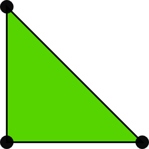
$$ \begin{align} \refphi_0(X,Y) &= 1 - X - Y\\ \refphi_1(X,Y) &= X\\ \refphi_2(X,Y) &= Y \end{align} $$
Higher-degree \( \refphi_r \) introduce more nodes (dof = node values)
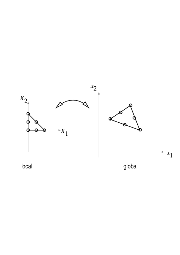
Mapping of local \( \X = (X,Y) \) coordinates in the reference cell to global, physical \( \x = (x,y) \) coordinates:
$$ \begin{equation} \x = \sum_{r} \refphi_r^{(1)}(\X)\xdno{q(e,r)} \label{fem:approx:fe:affine:map} \end{equation} $$
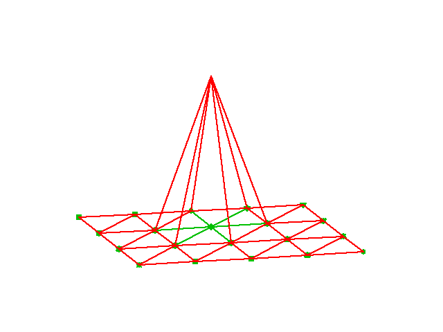
where
Idea: Use the basis functions of the element (not only the P1 functions) to map the element
$$ \begin{equation} \x = \sum_{r} \refphi_r(\X)\xdno{q(e,r)} \label{fem:approx:fe:isop:map} \end{equation} $$
Advantage: higher-order polynomial basis functions now map the reference cell to a curved triangle or tetrahedron.
Integrals must be transformed from \( \Omega^{(e)} \) (physical cell) to \( \tilde\Omega^r \) (reference cell):
$$ \begin{align} \int_{\Omega^{(e)}}\basphi_i (\x) \basphi_j (\x) \dx &= \int_{\tilde\Omega^r} \refphi_i (\X) \refphi_j (\X) \det J\, \dX\\ \int_{\Omega^{(e)}}\basphi_i (\x) f(\x) \dx &= \int_{\tilde\Omega^r} \refphi_i (\X) f(\x(\X)) \det J\, \dX \end{align} $$ where \( \dx = dx dy \) or \( \dx = dxdydz \) and \( \det J \) is the determinant of the Jacobian of the mapping \( \x(\X) \).
$$ \begin{equation} J = \left[\begin{array}{cc} \frac{\partial x}{\partial X} & \frac{\partial x}{\partial Y}\\ \frac{\partial y}{\partial X} & \frac{\partial y}{\partial Y} \end{array}\right], \quad \det J = \frac{\partial x}{\partial X}\frac{\partial y}{\partial Y} - \frac{\partial x}{\partial Y}\frac{\partial y}{\partial X} \label{fem:approx:fe:2D:mapping:J:detJ} \end{equation} $$
Affine mapping \eqref{fem:approx:fe:affine:map}: \( \det J=2\Delta \), \( \Delta = \hbox{cell volume} \)
!slide
Our aim is to extend the ideas for approximating \( f \) by \( u \), or solving
$$ u = f $$
to real differential equations like[[[
$$ -u'' + bu = f,\quad u(0)=1,\ u'(L)=D $$
Three methods are addressed:
$$ \begin{equation} \mathcal{L}(u) = 0,\quad x\in\Omega \end{equation} $$
Examples (1D problems):
$$ \begin{align} \mathcal{L}(u) &= \frac{d^2u}{dx^2} - f(x), \label{fem:deq:1D:L1}\\ \mathcal{L}(u) &= \frac{d}{dx}\left(\dfc(x)\frac{du}{dx}\right) + f(x), \label{fem:deq:1D:L2}\\ \mathcal{L}(u) &= \frac{d}{dx}\left(\dfc(u)\frac{du}{dx}\right) - au + f(x), \label{fem:deq:1D:L3}\\ \mathcal{L}(u) &= \frac{d}{dx}\left(\dfc(u)\frac{du}{dx}\right) + f(u,x) \label{fem:deq:1D:L4} \end{align} $$
$$ \begin{equation} {\cal B}_0(u)=0,\ x=0,\quad {\cal B}_1(u)=0,\ x=L \end{equation} $$
Examples:
$$ \begin{align} \mathcal{B}_i(u) &= u - g,\quad &\hbox{Dirichlet condition}\\ \mathcal{B}_i(u) &= -\dfc \frac{du}{dx} - g,\quad &\hbox{Neumann condition}\\ \mathcal{B}_i(u) &= -\dfc \frac{du}{dx} - h(u-g),\quad &\hbox{Robin condition} \end{align} $$
Much is similar to approximating a function (solving \( u=f \)), but two new topics are needed:
$$ \begin{equation} R = \mathcal{L}(u) = \mathcal{L}(\sum_j c_j \baspsi_j) \neq 0 \end{equation} $$
Goal: minimize \( R \) wrt \( \sequencei{c} \) (and hope it makes a small \( e \) too)
$$ R=R(c_0,\ldots,c_N; x)$$
Idea: minimize
$$ \begin{equation} E = ||R||^2 = (R,R) = \int_{\Omega} R^2 dx \end{equation} $$
Minimization wrt \( \sequencei{c} \) implies
$$ \begin{equation} \frac{\partial E}{\partial c_i} = \int_{\Omega} 2R\frac{\partial R}{\partial c_i} dx = 0\quad \Leftrightarrow\quad (R,\frac{\partial R}{\partial c_i})=0,\quad i\in\If \label{fem:deq:1D:LS:eq1} \end{equation} $$
\( N+1 \) equations for \( N+1 \) unknowns \( \sequencei{c} \)
Idea: make \( R \) orthogonal to \( V \),
$$ \begin{equation} (R,v)=0,\quad \forall v\in V \label{fem:deq:1D:Galerkin0} \end{equation} $$
This implies
$$ \begin{equation} (R,\baspsi_i)=0,\quad i\in\If \label{fem:deq:1D:Galerkin} \end{equation} $$
\( N+1 \) equations for \( N+1 \) unknowns \( \sequencei{c} \)
Generalization of the Galerkin method: demand \( R \) orthogonal to some space \( W \), possibly \( W\neq V \):
$$ \begin{equation} (R,v)=0,\quad \forall v\in W \label{fem:deq:1D:WRM0} \end{equation} $$
If \( \{w_0,\ldots,w_N\} \) is a basis for \( W \):
$$ \begin{equation} (R,w_i)=0,\quad i\in\If \label{fem:deq:1D:WRM} \end{equation} $$
Idea: demand \( R=0 \) at \( N+1 \) points
$$ \begin{equation} R(\xno{i}; c_0,\ldots,c_N)=0,\quad i\in\If \label{fem:deq:1D:collocation} \end{equation} $$
Note: The collocation method is a weighted residual method with delta functions as weights
$$ 0 = \int_\Omega R(x;c_0,\ldots,c_N) \delta(x-\xno{i})\dx = R(\xno{i}; c_0,\ldots,c_N)$$
$$ \begin{equation} \hbox{property of } \delta(x):\quad \int_{\Omega} f(x)\delta (x-\xno{i}) dx = f(\xno{i}),\quad \xno{i}\in\Omega \label{fem:deq:1D:Dirac} \end{equation} $$
$$ \begin{equation} -u''(x) = f(x),\quad x\in\Omega=[0,L],\quad u(0)=0,\ u(L)=0 \label{fem:deq:1D:model1b} \end{equation} $$
Basis functions:
$$ \begin{equation} \baspsi_i(x) = \sinL{i},\quad i\in\If \label{fem:deq:1D:ex:sines:psi} \end{equation} $$
The residual:
$$ \begin{align} R(x;c_0,\ldots,c_N) &= u''(x) + f(x),\nonumber\\ &= \frac{d^2}{dx^2}\left(\sum_{j\in\If} c_j\baspsi_j(x)\right) + f(x),\nonumber\\ &= -\sum_{j\in\If} c_j\baspsi_j''(x) + f(x) \label{fem:deq:1D:ex:sines:res} \end{align} $$
Since \( u(0)=u(L)=0 \) we must ensure that all \( \baspsi_i(0)=\baspsi_i(L)=0 \). Then
$$ u(0) = \sum_jc_j\baspsi_j(0) = 0,\quad u(L) = \sum_jc_j\baspsi_j(L) $$
$$ (R,\frac{\partial R}{\partial c_i}) = 0,\quad i\in\If $$
$$ \begin{equation} \frac{\partial R}{\partial c_i} = \frac{\partial}{\partial c_i} \left(\sum_{j\in\If} c_j\baspsi_j''(x) + f(x)\right) = \baspsi_i''(x) \end{equation} $$
Because: $$ \frac{\partial}{\partial c_i}\left(c_0\baspsi_0'' + c_1\baspsi_1'' + \cdots + c_{i-1}\baspsi_{i-1}'' + \color{blue}{c_i\baspsi_{i}''} + c_{i+1}\baspsi_{i+1}'' + \cdots + c_N\baspsi_N'' \right) = \baspsi_{i}'' $$
$$ \begin{equation} (\sum_j c_j \baspsi_j'' + f,\baspsi_i'')=0,\quad i\in\If \end{equation} $$
Rearrangement:
$$ \begin{equation} \sum_{j\in\If}(\baspsi_i'',\baspsi_j'')c_j = -(f,\baspsi_i''),\quad i\in\If \end{equation} $$
This is a linear system
$$ \begin{equation*} \sum_{j\in\If}A_{i,j}c_j = b_i,\quad i\in\If \end{equation*} $$ with
$$ \begin{align} A_{i,j} &= (\baspsi_i'',\baspsi_j'')\nonumber\\ & = \pi^4(i+1)^2(j+1)^2L^{-4}\int_0^L \sinL{i}\sinL{j}\, dx\nonumber\\ &= \left\lbrace \begin{array}{ll} {1\over2}L^{-3}\pi^4(i+1)^4 & i=j \\ 0, & i\neq j \end{array}\right. \\ b_i &= -(f,\baspsi_i'') = (i+1)^2\pi^2L^{-2}\int_0^Lf(x)\sinL{i}\, dx \end{align} $$
Useful property:
$$ \begin{equation} \int\limits_0^L \sinL{i}\sinL{j}\, dx = \delta_{ij},\quad \quad\delta_{ij} = \left\lbrace \begin{array}{ll} \half L & i=j \\ 0, & i\neq j \end{array}\right. \end{equation} $$
\( \Rightarrow\ (\baspsi_i'',\baspsi_j'') = \delta_{ij} \), i.e., diagonal \( A_{i,j} \), and we can easily solve for \( c_i \):
$$ \begin{equation} c_i = \frac{2L}{\pi^2(i+1)^2}\int_0^Lf(x)\sinL{i}\, dx \label{fem:deq:1D:ex:sines:solution} \end{equation} $$
Let's sympy do the work (\( f(x)=2 \)):
from sympy import *
import sys

i, j = symbols('i j', integer=True)
x, L = symbols('x L')
f = 2
a = 2*L/(pi**2*(i+1)**2)
c_i = a*integrate(f*sin((i+1)*pi*x/L), (x, 0, L))
c_i = simplify(c_i)
print c_i
$$ \begin{equation} c_i = 4 \frac{L^{2} \left(\left(-1\right)^{i} + 1\right)}{\pi^{3} \left(i^{3} + 3 i^{2} + 3 i + 1\right)},\quad u(x) = \sum_{k=0}^{N/2} \frac{8L^2}{\pi^3(2k+1)^3}\sinL{2k}\tp \end{equation} $$
Fast decay: \( c_2 = c_0/27 \), \( c_4=c_0/125 \) - only one term might be good enough:
$$ \begin{equation*} u(x) \approx \frac{8L^2}{\pi^3}\sin\left(\pi\frac{x}{L}\right)\tp \end{equation*} $$
\( R=u''+f \):
$$ \begin{equation*} (u''+f,v)=0,\quad \forall v\in V, \end{equation*} $$ or
$$ \begin{equation} (u'',v) = -(f,v),\quad\forall v\in V \end{equation} $$
This is a variational formulation of the differential equation problem.
\( \forall v\in V \) means for all basis functions:
$$ \begin{equation} (\sum_{j\in\If} c_j\baspsi_j'', \baspsi_i)=-(f,\baspsi_i),\quad i\in\If \end{equation} $$
Since \( \baspsi_i''\propto \baspsi_i \), Galerkin's method gives the same linear system and the same solution as the least squares method (in this particular example).
\( R=0 \) (i.e.,the differential equation) must be satisfied at \( N+1 \) points:
$$ \begin{equation} -\sum_{j\in\If} c_j\baspsi_j''(\xno{i}) = f(\xno{i}),\quad i\in\If \end{equation} $$
This is a linear system \( \sum_j A_{i,j}=b_i \) with entries
$$ \begin{equation*} A_{i,j}=-\baspsi_j''(\xno{i})= (j+1)^2\pi^2L^{-2}\sin\left((j+1)\pi \frac{x_i}{L}\right), \quad b_i=2 \end{equation*} $$
Choose: \( N=0 \), \( x_0=L/2 \)
$$ c_0=2L^2/\pi^2 $$
Second-order derivatives will hereafter be integrated by parts
$$ \begin{align} \int_0^L u''(x)v(x) dx &= - \int_0^Lu'(x)v'(x)dx + [vu']_0^L\nonumber\\ &= - \int_0^Lu'(x)v'(x) dx + u'(L)v(L) - u'(0)v(0) \label{fem:deq:1D:intbyparts} \end{align} $$
Motivation:
Dirichlet conditions: \( u(0)=C \) and \( u(L)=D \). Choose for example
$$ B(x) = \frac{1}{L}(C(L-x) + Dx):\qquad B(0)=C,\ B(L)=D $$
$$ \begin{equation} u(x) = B(x) + \sum_{j\in\If} c_j\baspsi_j(x), \label{fem:deq:1D:essBC:Bfunc:u1} \end{equation} $$
$$ u(0) = B(0)= C,\quad u(L) = B(L) = D $$
Dirichlet condition: \( u(L)=D \). Choose for example
$$ B(x) = D:\qquad B(L)=D $$
$$ \begin{equation} u(x) = B(x) + \sum_{j\in\If} c_j\baspsi_j(x), \label{fem:deq:1D:essBC:Bfunc:u1} \end{equation} $$
$$ u(L) = B(L) = D $$
The finite element literature (and much FEniCS documentation) applies an abstract notation for the variational formulation:
$$ a(u,v) = L(v)\quad \forall v\in V $$
$$ -u''=f, \quad u'(0)=C,\ u(L)=D,\quad u=D + \sum_jc_j\baspsi_j$$
Variational formulation:
$$ \int_{\Omega} u' v'dx = \int_{\Omega} fvdx\quad - v(0)C \hbox{or}\quad (u',v') = (f,v) - v(0)C \quad\forall v\in V $$
Abstract formulation: finn \( (u-B)\in V \) such that
$$ a(u,v) = L(v)\quad \forall v\in V$$
We identify
$$ a(u,v) = (u',v'),\quad L(v) = (f,v) -v(0)C $$
$$ L(\alpha_1 v_1 + \alpha_2 v_2) =\alpha_1 L(v_1) + \alpha_2 L(v_2), $$
Bilinear form means $$ \begin{align*} a(\alpha_1 u_1 + \alpha_2 u_2, v) &= \alpha_1 a(u_1,v) + \alpha_2 a(u_2, v), \\ a(u, \alpha_1 v_1 + \alpha_2 v_2) &= \alpha_1 a(u,v_1) + \alpha_2 a(u, v_2) \end{align*} $$
In nonlinear problems: Find \( (u-B)\in V \) such that \( F(u;v)=0\ \forall v\in V \)
$$ a(u,v) = L(v)\quad \forall v\in V\quad\Leftrightarrow\quad a(u,\baspsi_i) = L(\baspsi_i)\quad i\in\If$$
We can now derive the corresponding linear system once and for all:
$$ a(\sum_{j\in\If} c_j \baspsi_j,\baspsi_i)c_j = L(\baspsi_i)\quad i\in\If$$
Because of linearity,
$$ \sum_{j\in\If} \underbrace{a(\baspsi_j,\baspsi_i)}_{A_{i,j}}c_j = \underbrace{L(\baspsi_i)}_{b_i}\quad i\in\If$$
$$ A_{i,j} = a(\baspsi_j,\baspsi_i),\quad b_i = L(\baspsi_i) $$
If \( a(u,v)=a(v,u) \),
$$ a(u,v)=L(v)\quad\forall v\in V,$$
is equivalent to minimizing the functional
$$ F(v) = {\half}a(v,v) - L(v) $$ over all functions \( v\in V \). That is,
$$ F(u)\leq F(v)\quad \forall v\in V\tp $$
$$ \begin{equation} -\frac{d}{dx}\left( \dfc(x)\frac{du}{dx}\right) = f(x),\quad x\in\Omega =[0,L],\ u(0)=C,\ u(L)=D \end{equation} $$
$$ B(x) = C + \frac{1}{L}(D-C)x$$
$$ R = -\frac{d}{dx}\left( a\frac{du}{dx}\right) -f $$
Galerkin's method:
$$ (R, v) = 0,\quad \forall v\in V, $$
or with integrals:
$$ \int_{\Omega} \left(\frac{d}{dx}\left( \dfc\frac{du}{dx}\right) -f\right)v \dx = 0,\quad \forall v\in V \tp $$
Integration by parts:
$$ -\int_{\Omega} \frac{d}{dx}\left( \dfc(x)\frac{du}{dx}\right) v \dx = \int_{\Omega} \dfc(x)\frac{du}{dx}\frac{dv}{dx}\dx - \left[\dfc\frac{du}{dx}v\right]_0^L \tp $$
Boundary terms vanish since \( v(0)=v(L)=0 \)
Find \( (u-B)\in V \) such that
$$ \int_{\Omega} \dfc(x)\frac{du}{dx}\frac{dv}{dx}dx = \int_{\Omega} f(x)vdx,\quad \forall v\in V, $$
Compact notation:
$$ \underbrace{(\dfc u',v')}_{a(u,v)} = \underbrace{(f,v)}_{L(v)}, \quad \forall v\in V $$
With
$$ a(u,v) = (\dfc u', v),\quad L(v) = (f,v) $$
we can just use the formula for the linear system:
$$ \begin{align*} A_{i,j} &= a(\baspsi_j,\baspsi_i) = (\dfc \baspsi_j', \baspsi_i') = \int_\Omega \dfc \baspsi_j' \baspsi_i'\dx = \int_\Omega \baspsi_i' \dfc \baspsi_j'\dx = a(\baspsi_i,\baspsi_j) = A_{j,i}\\ b_i &= (f,\baspsi_i) = \int_\Omega f\baspsi_i\dx \end{align*} $$
\( v=\baspsi_i \) and \( u=B + \sum_jc_j\baspsi_j \):
$$ (\dfc B' + \dfc \sum_{j\in\If} c_j \baspsi_j', \baspsi_i') = (f,\baspsi_i), \quad i\in\If \tp $$
Reorder to form linear system:
$$ \sum_{j\in\If} (\dfc\baspsi_j', \baspsi_i')c_j = (f,\baspsi_i) + (a(D-C)L^{-1}, \baspsi_i'), \quad i\in\If \tp $$
This is \( \sum_j A_{i,j}c_j=b_i \) with
$$ \begin{align*} A_{i,j} &= (a\baspsi_j', \baspsi_i') = \int_{\Omega} \dfc(x)\baspsi_j'(x) \baspsi_i'(x)\dx\\ b_i &= (f,\baspsi_i) + (a(D-C)L^{-1},\baspsi_i')= \int_{\Omega} \left(f(x)\baspsi_i(x) + \dfc(x)\frac{D-C}{L}\baspsi_i'(x)\right) \dx \end{align*} $$
$$ \begin{equation} -u''(x) + bu'(x) = f(x),\quad x\in\Omega =[0,L],\ u(0)=C,\ u'(L)=E \end{equation} $$
New features:
$$ u = C + \sum_{j\in\If} c_j \baspsi_i(x)$$
Galerkin's method: multiply by \( v \), integrate over \( \Omega \), integrate by parts.
$$ (-u'' + bu' - f, v) = 0,\quad\forall v\in V$$
$$ (u',v') + (bu',v) = (f,v) + [u' v]_0^L, \quad\forall v\in V$$
Now, \( [u' v]_0^L = u'(L)v(L) = E v(L) \) because \( v(0)=0 \) and \( u'(L)=E \):
$$ (u'v') + (bu',v) = (f,v) + Ev(L), \quad\forall v\in V$$
$$ (u'v') + (bu',v) = (f,v) + Ev(L), \quad\forall v\in V,$$
Important:
Abstract notation:
$$ a(u,v)=L(v)\quad\forall v\in V$$
Here:
$$ \begin{align*} a(u,v)&=(u',v') + (bu',v)\\ L(v)&= (f,v) + E v(L) \end{align*} $$
Insert \( u=C+\sum_jc_j\baspsi_j \) and \( v=\baspsi_i \):
$$ \sum_{j\in\If} \underbrace{((\baspsi_j',\baspsi_i') + (b\baspsi_j',\baspsi_i))}_{A_{i,j}} c_j = \underbrace{(f,\baspsi_i) + E \baspsi_i(L)}_{b_i} $$
Observation: \( A_{i,j} \) is not symmetric because of the term
$$ (b\baspsi_j',\baspsi_i)=\int_{\Omega} b\baspsi_j'\baspsi_i dx \neq \int_{\Omega} b \baspsi_i' \baspsi_jdx = (\baspsi_i',b\baspsi_j) $$
$$ (u',v') + (bu',v) = (f,v) + u'(L)v(L) - u'(0)v(0)$$
Problem:
$$ \begin{equation} -(\dfc(u)u')' = f(u),\quad x\in [0,L],\ u(0)=0,\ u'(L)=E \end{equation} $$
Galerkin: multiply by \( v \), integrate, integrate by parts
$$ \int_0^L \dfc(u)\frac{du}{dx}\frac{dv}{dx}\dx = \int_0^L f(u)v\dx + [\dfc(u)vu']_0^L\quad\forall v\in V $$
or
$$ (\dfc(u)u', v') = (f(u),v) + \dfc(u(L))v(L)E\quad\forall v\in V $$
$$ \begin{equation*} -u''(x)=f(x),\quad x\in \Omega=[0,1],\quad u'(0)=C,\ u(1)=D \end{equation*} $$
$$ A_{i,j} = (\baspsi_j',\baspsi_i') = \int_{0}^1 \baspsi_i'(x)\baspsi_j'(x)dx = \int_0^1 (i+1)(j+1)(1-x)^{i+j} dx, $$
Choose \( f(x)=2 \):
$$ \begin{align*} b_i &= (2,\baspsi_i) - (D,\baspsi_i') -C\baspsi_i(0)\\ &= \int_0^1 \left( 2(1-x)^{i+1} - D(i+1)(1-x)^i\right)dx -C\baspsi_i(0) \end{align*} $$
Can easily do the integrals with sympy. \( N=1 \):
$$ \begin{equation*} \left(\begin{array}{cc} 1 & 1\\ 1 & 4/3 \end{array}\right) \left(\begin{array}{c} c_0\\ c_1 \end{array}\right) = \left(\begin{array}{c} -C+D+1\\ 2/3 -C + D \end{array}\right) \end{equation*} $$
$$ c_0=-C+D+2, \quad c_1=-1,$$
$$ u(x) = 1 -x^2 + D + C(x-1)\quad\hbox{(exact solution)} $$
Assume that apart from boundary conditions, \( \uex \) lies in the same space \( V \) as where we seek \( u \):
$$ \begin{align*} u &= B + F,\quad F\in V a(B+F, v) &= L(v)\quad\forall v\in V \uex & = B + E,\quad E\in V a(B+E, v) &= L(v)\quad\forall v\in V \end{align*} $$
Subtract: \( a(F-E,v)=0\ \Rightarrow\ E=F \) and \( u = \uex \)
Tasks:
$$ -u''(x) = 2,\quad x\in (0,L),\ u(0)=u(L)=0,$$
Variational formulation:
$$ (u',v') = (2,v)\quad\forall v\in V $$
Since \( u(0)=0 \) and \( u(L)=0 \), we must force
$$ v(0)=v(L)=0,\quad \baspsi_i(0)=\baspsi_i(L)=0$$
Use finite element basis, but exclude \( \basphi_0 \) and \( \basphi_{N_n} \) since these are not 0 on the boundary:
$$ \baspsi_i=\basphi_{i+1},\quad i=0,\ldots,N=N_n-2$$
Introduce index mapping \( \nu(j) \): \( \baspsi_i = \basphi_{\nu(i)} \)
$$ u = \sum_{j\in\If}c_j\basphi_{\nu(i)},\quad i=0,\ldots,N,\quad \nu(j) = j+1$$
Irregular numbering: more complicated \( \nu(j) \) table
$$ \begin{equation*} A_{i,j}=\int_0^L\basphi_{i+1}'(x)\basphi_{j+1}'(x) dx,\quad b_i=\int_0^L2\basphi_{i+1}(x) dx \end{equation*} $$
Many will prefer to change indices to obtain a \( \basphi_i'\basphi_j' \) product: \( i+1\rightarrow i \), \( j+1\rightarrow j \)
$$ \begin{equation*} A_{i-1,j-1}=\int_0^L\basphi_{i}'(x)\basphi_{j}'(x) \dx,\quad b_{i-1}=\int_0^L2\basphi_{i}(x) \dx \end{equation*} $$
$$ \basphi_i = \pm h^{-1} $$
$$ A_{i-1,i-1} = h^{-2}2h = 2h^{-1},\quad A_{i-1,i-2} = h^{-1}(-h^{-1})h = -h^{-1},\quad A_{i-1,i}=A_{i-1,i-2}$$
$$ b_{i-1} = 2({\half}h + {\half}h) = 2h$$
$$ \begin{equation} \frac{1}{h}\left( \begin{array}{ccccccccc} 2 & -1 & 0 &\cdots & \cdots & \cdots & \cdots & \cdots & 0 \\ -1 & 2 & -1 & \ddots & & & & & \vdots \\ 0 & -1 & 2 & -1 & \ddots & & & & \vdots \\ \vdots & \ddots & & \ddots & \ddots & 0 & & & \vdots \\ \vdots & & \ddots & \ddots & \ddots & \ddots & \ddots & & \vdots \\ \vdots & & & 0 & -1 & 2 & -1 & \ddots & \vdots \\ \vdots & & & & \ddots & \ddots & \ddots &\ddots & 0 \\ \vdots & & & & &\ddots & \ddots &\ddots & -1 \\ 0 &\cdots & \cdots &\cdots & \cdots & \cdots & 0 & -1 & 2 \end{array} \right) \left( \begin{array}{c} c_0 \\ \vdots\\ \vdots\\ \vdots \\ \vdots \\ \vdots \\ \vdots \\ \vdots\\ c_{N} \end{array} \right) = \left( \begin{array}{c} 2h \\ \vdots\\ \vdots\\ \vdots \\ \vdots \\ \vdots \\ \vdots \\ \vdots\\ 2h \end{array} \right) \label{fem:deq:1D:ex1:Ab:glob} \end{equation} $$
The standard finite difference method for \( -u''=2 \) is
$$ -\frac{1}{h^2}u_{i-1} + \frac{2}{h^2}u_{i} - \frac{1}{h^2}u_{i+1} = 2 $$
(Remains to study the equations involving boundary values)
$$ \refphi_0(X)=\half(1-X),\quad\refphi_1(X)=\half(1+X)$$
$$ \frac{d\refphi_0}{dX} = -\half,\quad \frac{d\refphi_1}{dX} = \half $$
From the chain rule
$$ \frac{d\refphi_r}{dx} = \frac{d\refphi_r}{dX}\frac{dX}{dx} = \frac{2}{h}\frac{d\refphi_r}{dX}$$
$$ \begin{equation*} A_{i-1,j-1}^{(e)}=\int_{\Omega^{(e)}} \basphi_i'(x)\basphi_j'(x) \dx = \int_{-1}^1 \frac{2}{h}\frac{d\refphi_r}{dX}\frac{2}{h}\frac{d\refphi_s}{dX} \frac{h}{2} \dX = \tilde A_{r,s}^{(e)} \end{equation*} $$
$$ \begin{equation*} b_{i-1}^{(e)} = \int_{\Omega^{(e)}} 2\basphi_i(x) \dx = \int_{-1}^12\refphi_r(X)\frac{h}{2} \dX = \tilde b_{r}^{(e)}, \quad i=q(e,r),\ r=0,1 \end{equation*} $$
Must run through all \( r,s=0,1 \) and \( r=0,1 \) and compute each entry in the element matrix and vector:
$$ \begin{equation} \tilde A^{(e)} =\frac{1}{h}\left(\begin{array}{rr} 1 & -1\\ -1 & 1 \end{array}\right),\quad \tilde b^{(e)} = h\left(\begin{array}{c} 1\\ 1 \end{array}\right)\tp \label{fem:deq:1D:ex1:Ab:elm} \end{equation} $$
Example:
$$ \tilde A^{(e)}_{0,1} = \int_{-1}^1 \frac{2}{h}\frac{d\refphi_0}{dX}\frac{2}{h}\frac{d\refphi_1}{dX} \frac{h}{2} \dX = \frac{2}{h}(-\half)\frac{2}{h}\half\frac{h}{2} \int_{-1}^1\dX = -\frac{1}{h} $$
$$ \tilde A^{(e)} =\frac{1}{h}\left(\begin{array}{r} 1 \end{array}\right),\quad \tilde b^{(e)} = h\left(\begin{array}{c} 1 \end{array}\right) $$
Only one degree of freedom ("node") in these cells (\( r=0 \) counts the only dof)
4 P1 elements:
vertices = [0, 0.5, 1, 1.5, 2]
cells = [[0, 1], [1, 2], [2, 3], [3, 4]]
dof_map = [[0], [0, 1], [1, 2], [2]]       # only 1 dof in elm 0, 3
Python code for the assembly algorithm:
# Ae[e][r,s]: element matrix, be[e][r]: element vector
# A[i,j]: coefficient matrix, b[i]: right-hand side

for e in range(len(Ae)):
    for r in range(Ae[e].shape[0]):
        for s in range(Ae[e].shape[1]):
            A[dof_map[e,r],dof_map[e,s]] += Ae[e][i,j]
        b[dof_map[e,r]] += be[e][i,j]
Result: same linear system as arose from computations in the physical domain
Suppose we have a Dirichlet condition \( u(\xno{k})=U_k \), \( k\in\Ifb \):
$$ u(\xno{k}) = \sum_{j\in\Ifb} U_j\underbrace{\basphi_j(x)}_{\neq 0 \hbox{ only for }j=k} + \sum_{j\in\If} c_j\underbrace{\basphi_{\nu(j)}(\xno{k})}_{=0,\ k\not\in\If} = U_k $$
$$ -u''=2, \quad u(0)=C,\ u(L)=D $$
$$ \int_0^L u'v'\dx = \int_0^L2v\dx\quad\forall v\in V$$
$$ (u',v') = (2,v)\quad\forall v\in V$$
$$ \begin{equation} B(x) = \sum_{j\in\Ifb} U_j\basphi_j(x) \end{equation} $$
Here \( \Ifb = \{0,N_n\} \), \( U_0=C \), \( U_{N_n}=D \),
$$ \baspsi_i = \basphi_{\nu(i)}, \quad \nu(i)=i+1,\quad i\in\If = \{0,\ldots,N=N_n-2\} $$
$$ \begin{equation} u(x) = C\basphi_0(x) + D\basphi_{N_n}(x) + \sum_{j\in\If}c_j\basphi_{\nu(j)} \end{equation} $$
Insert \( u = B + \sum_j c_j\baspsi_j \) in variational formulation:
$$ (u',v') = (2,v)\quad\Rightarrow\quad (\sum_jc_j\baspsi_j',\baspsi_i') = (2-B',\baspsi_i)\quad \forall v\in V$$
$$ \begin{align*} u(x) &= \underbrace{C\cdot\basphi_0 + D\basphi_{N_n}}_{B(x)} + \sum_{j\in\If} c_j\basphi_{j+1}\\ &= C\cdot\basphi_0 + D\basphi_{N_n} + c_0\basphi_1 + c_1\basphi_2 +\cdots + c_N\basphi_{N_n-1} \end{align*} $$
$$ A_{i-1,j-1} = \int_0^L \basphi_i'(x)\basphi_j'(x) \dx,\quad b_{i-1} = \int_0^L (f(x) - C\basphi_{0}'(x) - D\basphi_{N_n}'(x)) \basphi_i(x) \dx $$ for \( i,j = 1,\ldots,N+1=N_n-1 \).
New boundary terms from \( -\int B'\basphi_i\dx \): \( C/2 \) for \( i=1 \) and \( -D/2 \) for \( i=N_n-1 \)
$$ \tilde b_0^{(N_e)} = \int_{-1}^1 \left(f - D\frac{2}{h} \frac{d\refphi_1}{dX}\right) \refphi_0\frac{h}{2} \dX = (\frac{h}{2}(2 - D\frac{2}{h}\half) \int_{-1}^1 \refphi_0 \dX = h - D/2 $$
From the first cell:
$$ \tilde b_0^{(0)} = \int_{-1}^1 \left(f - C\frac{2}{h} \frac{d\refphi_0}{dX}\right) \refphi_1\frac{h}{2} \dX = (\frac{h}{2}(2 + C\frac{2}{h}\half) \int_{-1}^1 \refphi_1 \dX = h + C/2\tp $$
$$ \begin{equation} u(x) = \sum_{j\in\If}c_j\basphi_j(x),\quad \If=\{0,\ldots,N=N_n\} \label{fem:deq:1D:fem:essBC:Bfunc:modsys:uall} \end{equation} $$
$$ -u''=2,\quad u(0)=0,\ u(L)=D$$
Assemble as if there were no Dirichlet conditions:
$$ \begin{equation} \frac{1}{h}\left( \begin{array}{ccccccccc} 1 & -1 & 0 &\cdots & \cdots & \cdots & \cdots & \cdots & 0 \\ -1 & 2 & -1 & \ddots & & & & & \vdots \\ 0 & -1 & 2 & -1 & \ddots & & & & \vdots \\ \vdots & \ddots & & \ddots & \ddots & 0 & & & \vdots \\ \vdots & & \ddots & \ddots & \ddots & \ddots & \ddots & & \vdots \\ \vdots & & & 0 & -1 & 2 & -1 & \ddots & \vdots \\ \vdots & & & & \ddots & \ddots & \ddots &\ddots & 0 \\ \vdots & & & & &\ddots & \ddots &\ddots & -1 \\ 0 &\cdots & \cdots &\cdots & \cdots & \cdots & 0 & -1 & 1 \end{array} \right) \left( \begin{array}{c} c_0 \\ \vdots\\ \vdots\\ \vdots \\ \vdots \\ \vdots \\ \vdots \\ \vdots\\ c_{N} \end{array} \right) = \left( \begin{array}{c} h \\ 2h\\ \vdots\\ \vdots \\ \vdots \\ \vdots \\ \vdots \\ 2h\\ h \end{array} \right) \label{fem:deq:1D:ex1:Ab:glob2} \end{equation} $$
In cell 0 we know \( u \) for local node (degree of freedom) \( r=0 \). Replace the first cell equation by \( \tilde c_0 = 0 \):
$$ \begin{equation} \tilde A^{(0)} = A = \frac{1}{h}\left(\begin{array}{rr} h & 0\\ -1 & 1 \end{array}\right),\quad \tilde b^{(0)} = \left(\begin{array}{c} 0\\ h \end{array}\right) \label{fem:deq:1D:ex1:Ab:elm:bc:0} \end{equation} $$
In cell \( N_e \) we know \( u \) for local node \( r=1 \). Replace the last equation in the cell system by \( \tilde c_1=D \):
$$ \begin{equation} \tilde A^{(N_e)} = A = \frac{1}{h}\left(\begin{array}{rr} 1 & -1\\ 0 & h \end{array}\right),\quad \tilde b^{(N_e)} = \left(\begin{array}{c} h\\ D \end{array}\right) \label{fem:deq:1D:ex1:Ab:elm:bc:N} \end{equation} $$
$$ \begin{equation} \frac{1}{h}\left( \begin{array}{ccccccccc} 1 & 0 & 0 &\cdots & \cdots & \cdots & \cdots & \cdots & 0 \\ 0 & 2 & -1 & \ddots & & & & & \vdots \\ 0 & -1 & 2 & -1 & \ddots & & & & \vdots \\ \vdots & \ddots & & \ddots & \ddots & 0 & & & \vdots \\ \vdots & & \ddots & \ddots & \ddots & \ddots & \ddots & & \vdots \\ \vdots & & & 0 & -1 & 2 & -1 & \ddots & \vdots \\ \vdots & & & & \ddots & \ddots & \ddots &\ddots & 0 \\ \vdots & & & & &\ddots & \ddots &\ddots & 0 \\ 0 &\cdots & \cdots &\cdots & \cdots & \cdots & 0 & 0 & 1 \end{array} \right) \left( \begin{array}{c} c_0 \\ \vdots\\ \vdots\\ \vdots \\ \vdots \\ \vdots \\ \vdots \\ \vdots\\ c_{N} \end{array} \right) = \left( \begin{array}{c} 0 \\ 2h\\ \vdots\\ \vdots \\ \vdots \\ \vdots \\ \vdots \\ 2h +D/h\\ D \end{array} \right) \label{fem:deq:1D:ex1:Ab:glob3:symm} \end{equation} $$
Symmetric modification applied to \( \tilde A^{(N_e)} \):
$$ \begin{equation} \tilde A^{(N_e)} = A = \frac{1}{h}\left(\begin{array}{rr} 1 & 0\\ 0 & 1 \end{array}\right),\quad \tilde b^{(N-1)} = \left(\begin{array}{c} h + D/h\\ D \end{array}\right) \label{fem:deq:1D:ex1:Ab:elm:bc:N:symm} \end{equation} $$
$$ -u''=f,\quad u'(0)=C,\ u(L)=D$$
Galerkin's method:
$$ \begin{equation*} \int_0^L(u''(x)+f(x))\baspsi_i(x) dx = 0,\quad i\in\If \end{equation*} $$
Integration of \( u''\baspsi_i \) by parts:
$$ \begin{equation*} \int_0^Lu'(x)\baspsi_i'(x) \dx -(u'(L)\baspsi_i(L) - u'(0)\baspsi_i(0)) - \int_0^L f(x)\baspsi_i(x) \dx =0, \quad i\in\If \end{equation*} $$
$$ \begin{equation} \sum_{j=0}^{N=N_n-1}\left( \int_0^L \basphi_i'(x)\basphi_j'(x) dx \right)c_j = \int_0^L\left(f(x)\basphi_i(x) -D\basphi_N'(x)\basphi_i(x)\right) dx - C\basphi_i(0) \label{fem:deq:1D:natBC} \end{equation} $$ for \( i=0,\ldots,N=N_n-1 \).
$$ \begin{equation*} u(x) = \sum_{j=0}^{N=N_n} c_j\basphi_j(x) \end{equation*} $$
$$ \begin{equation} \sum_{j=0}^{N=N_n}\left( \int_0^L \basphi_i'(x)\basphi_j'(x) dx \right)c_j = \int_0^L f(x)\basphi_i(x)\basphi_i(x) dx - C\basphi_i(0) \label{fem:deq:1D:natBC} \end{equation} $$
Assemble entries for \( i=0,\ldots,N=N_n \) and then modify the last equation to \( c_N=D \)
The extra term \( C\basphi_0(0) \) affects only the element vector from the first cells since \( \basphi_0=0 \) on all other cells.
$$ \begin{equation} \tilde A^{(0)} = A = \frac{1}{h}\left(\begin{array}{rr} 1 & 1\\ -1 & 1 \end{array}\right),\quad \tilde b^{(0)} = \left(\begin{array}{c} h - C\\ h \end{array}\right) \label{fem:deq:1D:ex1:Ab:elm:bc:nat} \end{equation} $$
The differential equation problem defines the integrals in the variational formulation.
Request these functions from the user:
integrand_lhs(phi, r, s, x)
boundary_lhs(phi, r, s, x)
integrand_rhs(phi, r, x)
boundary_rhs(phi, r, x)
Must also have a mesh with vertices, cells, and dof_map
<Declare global matrix, global rhs: A, b>

# Loop over all cells
for e in range(len(cells)):

    # Compute element matrix and vector
    n = len(dof_map[e])  # no of dofs in this element
    h = vertices[cells[e][1]] - vertices[cells[e][0]]
    <Declare element matrix, element vector: A_e, b_e>

    # Integrate over the reference cell
    points, weights = <numerical integration rule>
    for X, w in zip(points, weights):
        phi = <basis functions + derivatives at X>
        detJ = h/2
        x = <affine mapping from X>
        for r in range(n):
            for s in range(n):
                A_e[r,s] += integrand_lhs(phi, r, s, x)*detJ*w
            b_e[r] += integrand_rhs(phi, r, x)*detJ*w

    # Add boundary terms
    for r in range(n):
        for s in range(n):
            A_e[r,s] += boundary_lhs(phi, r, s, x)*detJ*w
        b_e[r] += boundary_rhs(phi, r, x)*detJ*w
for e in range(len(cells)):
    ...

    # Incorporate essential boundary conditions
    for r in range(n):
        global_dof = dof_map[e][r]
        if global_dof in essbc_dofs:
            # dof r is subject to an essential condition
            value = essbc_docs[global_dof]
            # Symmetric modification
            b_e -= value*A_e[:,r]
            A_e[r,:] = 0
            A_e[:,r] = 0
            A_e[r,r] = 1
            b_e[r] = value

    # Assemble
    for r in range(n):
        for s in range(n):
            A[dof_map[e][r], dof_map[e][r]] += A_e[r,s]
        b[dof_map[e][r] += b_e[r]

<solve linear system>
$$ \begin{equation} -\int_{\Omega} \nabla\cdot (a(\x)\nabla u) v\dx = \int_{\Omega} a(\x)\nabla u\cdot\nabla v \dx - \int_{\partial\Omega} a\frac{\partial u}{\partial n} v \ds \label{fem:deq:2D:int:by:parts} \end{equation} $$
$$ \begin{align} \v\cdot\nabla u + \alpha u &= \nabla\cdot\left( a\nabla u\right) + f, \quad & \x\in\Omega\\ u &= u_0,\quad &\x\in\partial\Omega_D\\ -a\frac{\partial u}{\partial n} &= g,\quad &\x\in\partial\Omega_N \end{align} $$
$$ u(\x) = B(\x) + \sum_{j\in\If} c_j\baspsi_j(\x),\quad B(\x)=u_0(\x) $$
Galerkin's method: multiply by \( v\in V \) and integrate over \( \Omega \),
$$ \int_{\Omega} (\v\cdot\nabla u + \alpha u)v\dx = \int_{\Omega} \nabla\cdot\left( a\nabla u\right)\dx + \int_{\Omega}fv \dx $$
Integrate second-order term by parts:
$$ \int_{\Omega} \nabla\cdot\left( a\nabla u\right) v \dx = -\int_{\Omega} a\nabla u\cdot\nabla v\dx + \int_{\partial\Omega} a\frac{\partial u}{\partial n} v\ds, $$
Resulting variational form:
$$ \int_{\Omega} (\v\cdot\nabla u + \alpha u)v\dx = -\int_{\Omega} a\nabla u\cdot\nabla v\dx + \int_{\partial\Omega} a\frac{\partial u}{\partial n} v\ds + \int_{\Omega} fv \dx $$
Note: \( v\neq 0 \) only on \( \partial\Omega_N \):
$$ \int_{\partial\Omega} a\frac{\partial u}{\partial n} v\ds = \int_{\partial\Omega_N} \underbrace{a\frac{\partial u}{\partial n}}_{-g} v\ds = -\int_{\partial\Omega_N} gv\ds $$
The final variational form:
$$ \int_{\Omega} (\v\cdot\nabla u + \alpha u)v\dx = -\int_{\Omega} a\nabla u\cdot\nabla v \dx - \int_{\partial\Omega_N} g v\ds + \int_{\Omega} fv \dx $$
Or with inner product notation:
$$ (\v\cdot\nabla u, v) + (\alpha u,v) = - (a\nabla u,\nabla v) - (g,v)_{N} + (f,v) $$
\( (g,v)_{N} \): line or surface integral over \( \partial\Omega_N \).
$$ u = B + \sum_{j\in\If} c_j\baspsi_j,\quad B = u_0 $$
$$ A_{i,j} = (\v\cdot\nabla \baspsi_j, \baspsi_i) + (\alpha \baspsi_j ,\baspsi_i) + (a\nabla \baspsi_j,\nabla \baspsi_i) $$
$$ b_i = (g,\baspsi_i)_{N} + (f,\baspsi_i) - (\v\cdot\nabla u_0, \baspsi_i) + (\alpha u_0 ,\baspsi_i) + (a\nabla u_0,\nabla \baspsi_i) $$
$$ \begin{equation} \int_{{\Omega}^{(e)}} a(\x)\nabla\basphi_i\cdot\nabla\basphi_j\dx \end{equation} $$
Mapping from reference to physical coordinates:
$$ \x(\X) $$
with Jacobian \( J \),
$$ J_{i,j}=\frac{\partial x_j}{\partial X_i} $$
Can derive
$$ \begin{align*} \nabla_{\X}\refphi_r &= J\cdot\nabla_{\x}\basphi_i\\ \nabla_{\x}\basphi_i &= \nabla_{\x}\refphi_r(\X) = J^{-1}\cdot\nabla_{\X}\refphi_r(\X) \end{align*} $$
Integral transformation from physical to reference coordinates:
$$ \begin{equation} \int_{\Omega^{(e)}} a(\x)\nabla_{\x}\basphi_i\cdot\nabla_{\x}\basphi_j\dx = \int_{\tilde\Omega^r} a(\x(\X))(J^{-1}\cdot\nabla_{\X}\refphi_r)\cdot (J^{-1}\cdot\nabla\refphi_s)\det J\dX \end{equation} $$
Numerical integration over reference cell triangles and tetrahedra:
$$ \int_{\tilde\Omega^r} g\dX = \sum_{j=0}^{n-1} w_j g(\bar\X_j)$$
Module numint.py contains different rules:
>>> import numint
>>> x, w = numint.quadrature_for_triangles(num_points=3)
>>> x
[(0.16666666666666666, 0.16666666666666666),
 (0.66666666666666666, 0.16666666666666666),
 (0.16666666666666666, 0.66666666666666666)]
>>> w
[0.16666666666666666, 0.16666666666666666, 0.16666666666666666]
$$ \begin{align} \frac{\partial u}{\partial t} &= \dfc\nabla^2 u + f(\x, t),\quad &\x\in\Omega, t\in (0,T] \label{fem:deq:diffu:eq}\\ u(\x, 0) & = I(\x),\quad &\x\in\Omega \label{fem:deq:diffu:ic}\\ \frac{\partial u}{\partial n} &= 0,\quad &\x\in\partial\Omega,\ t\in (0,T] \label{fem:deq:diffu:bcN} \end{align} $$
$$ \begin{equation} [D_t^+ u = \dfc\nabla^2 u + f]^n,\quad n=1,2,\ldots,N_t-1 \end{equation} $$
Solving wrt \( u^{n+1} \):
$$ \begin{equation} u^{n+1} = u^n + \Delta t \left( \dfc\nabla^2 u^n + f(\x, t_n)\right) \label{fem:deq:diffu:FE:eq:unp1} \end{equation} $$
$$ \begin{equation} \uex^{n+1} = \uex^n + \Delta t \left( \dfc\nabla^2 \uex^n + f(\x, t_n)\right) \label{fem:deq:diffu:FE:eq:uex:n} \end{equation} $$
$$ \uex^n \approx u^n = \sum_{j=0}^{N} c_j^{n}\baspsi_j(\x),\quad \uex^{n+1} \approx u^{n+1} = \sum_{j=0}^{N} c_j^{n+1}\baspsi_j(\x) $$
$$ R = u^{n+1} - u^n - \Delta t \left( \dfc\nabla^2 u^n + f(\x, t_n)\right)$$
$$ R = u^{n+1} - u^n - \Delta t \left( \dfc\nabla^2 u^n + f(\x, t_n)\right)$$
The weighted residual principle:
$$ \int_\Omega Rw\dx = 0,\quad \forall w\in W$$
results in
$$ \int_\Omega \left\lbrack u^{n+1} - u^n - \Delta t \left( \dfc\nabla^2 u^n + f(\x, t_n)\right) \right\rbrack w \dx =0, \quad \forall w \in W $$
Galerkin: \( W=V \), \( w=v \)
Isolating the unknown \( u^{n+1} \) on the left-hand side:
$$ \int_{\Omega} u^{n+1}\baspsi_i\dx = \int_{\Omega} \left\lbrack u^n - \Delta t \left( \dfc\nabla^2 u^n + f(\x, t_n)\right) \right\rbrack v\dx $$
Integration by parts of \( \int\dfc(\nabla^2 u^n) v\dx \):
$$ \int_{\Omega}\dfc(\nabla^2 u^n)v \dx = -\int_{\Omega}\dfc\nabla u^n\cdot\nabla v\dx + \underbrace{\int_{\partial\Omega}\dfc\frac{\partial u^n}{\partial n}v \dx}_{=0\quad\Leftarrow\quad\partial u^n/\partial n=0} $$
Variational form:
$$ \begin{equation} \int_{\Omega} u^{n+1} v\dx = \int_{\Omega} u^n v\dx - \Delta t \int_{\Omega}\dfc\nabla u^n\cdot\nabla v\dx + \Delta t\int_{\Omega}f^n v\dx,\quad\forall v\in V \label{fem:deq:diffu:FE:vf:u:np1} \end{equation} $$
u: the spatial unknown function to be computedu_1: the spatial function at the previous time level \( t-\Delta t \)u_2: the spatial function at \( t-2\Delta t \)or shorter
$$ \begin{equation} (u, \baspsi_i) = (u_1,v) - \Delta t (\dfc\nabla u_1,\nabla v) + (f^n, v) \label{fem:deq:diffu:FE:vf:u:short} \end{equation} $$
Insert these in
$$ (u, \baspsi_i) = (u_1,\baspsi_i) - \Delta t (\dfc\nabla u_1,\nabla\baspsi_i) + (f^n,\baspsi_i) $$
and order terms as matrix-vector products:
$$ \begin{equation} \sum_{j=0}^{N} \underbrace{(\baspsi_i,\baspsi_j)}_{M_{i,j}} c_j = \sum_{j=0}^{N} \underbrace{(\baspsi_i,\baspsi_j)}_{M_{i,j}} c_{1,j} -\Delta t \sum_{j=0}^{N} \underbrace{(\nabla\baspsi_i,\dfc\nabla\baspsi_j)}_{K_{i,j}} c_{1,j} + (f^n,\baspsi_i),\quad i=0,\ldots,N \end{equation} $$
$$ \begin{equation} Mc = Mc_1 - \Delta t Kc_1 + f \end{equation} $$
$$ \begin{align*} M &= \{M_{i,j}\},\quad M_{i,j}=(\baspsi_i,\baspsi_j),\quad i,j\in\If\\ K &= \{K_{i,j}\},\quad K_{i,j}=(\nabla\baspsi_i,\dfc\nabla\baspsi_j),\quad i,j\in\If\\ f &= \{(f(\x,t_n),\baspsi_i)\}_{i\in\If}\\ c &= \{c_i\}_{i\in\If}\\ c_1 &= \{c_{1,i}\}_{i\in\If} \end{align*} $$
Diffusion equation with finite elements is equivalent to
$$ \begin{equation} [D_t^+(u + \frac{1}{6}h^2D_xD_x u) = \dfc D_xD_x u + f]^n_i \label{fem:deq:diffu:FE:fdinterp} \end{equation} $$
Can lump the mass matrix by Trapezoidal integration and get the standard finite difference scheme
$$ \begin{equation} [D_t^+u = \dfc D_xD_x u + f]^n_i \end{equation} $$
Backward Euler scheme in time:
$$ [D_t^- u = \dfc\nabla^2 u + f(\x, t)]^n \tp $$
$$ \begin{equation} \uex^{n} - \Delta t \left( \dfc\nabla^2 \uex^n + f(\x, t_{n})\right) = \uex^{n-1} \label{fem:deq:diffu:BE:eq:un} \end{equation} $$
$$ \uex^n \approx u^n = \sum_{j=0}^{N} c_j^{n}\baspsi_j(\x),\quad \uex^{n+1} \approx u^{n+1} = \sum_{j=0}^{N} c_j^{n+1}\baspsi_j(\x)$$
$$ \begin{equation} \int_{\Omega} \left( u^{n}v + \Delta t \dfc\nabla u^n\cdot\nabla v\right)\dx = \int_{\Omega} u^{n-1} v\dx - \Delta t\int_{\Omega}f^n v\dx,\quad\forall v\in V \label{fem:deq:diffu:BE:vf:u:n} \end{equation} $$
or
$$ \begin{equation} (u,v) + \Delta t (\dfc\nabla u,\nabla v) = (u_1,v) + \Delta t (f^n,\baspsi_i) \label{fem:deq:diffu:BE:vf:u:short} \end{equation} $$
The linear system: insert \( u=\sum_j c_j\baspsi_i \) and \( u_1=\sum_j c_{1,j}\baspsi_i \),
$$ \begin{equation} (M + \Delta t \dfc K)c = Mc_1 + f \label{fem:deq:diffu:BE:vf:linsys} \end{equation} $$
Can interpret the resulting equation system as
$$ \begin{equation} [D_t^-(u + \frac{1}{6}h^2D_xD_x u) = \dfc D_xD_x u + f]^n_i \label{fem:deq:diffu:BE:fdinterp} \end{equation} $$
Lumped mass matrix (by Trapezoidal integration) gives a standard finite difference method:
$$ \begin{equation} [D_t^- u = \dfc D_xD_x u + f]^n_i \label{fem:deq:diffu:BE:fdinterp:lumped} \end{equation} $$
Dirichlet condition at \( x=0 \) and Neumann condition at \( x=L \):
$$ \begin{align} u(\x,t) &= u_0(\x,t),\quad & \x\in\partial\Omega_D\\ -\dfc\frac{\partial}{\partial n} u(\x,t) &= g(\x,t),\quad & \x\in\partial{\Omega}_N \end{align} $$
Forward Euler in time, Galerkin's method, and integration by parts:
$$ \begin{equation} \int_\Omega u^{n+1}v\dx = \int_\Omega (u^n - \Delta t\dfc\nabla u^n\cdot\nabla v)\dx - \Delta t\int_{\partial\Omega_N} gv\ds,\quad \forall v\in V \end{equation} $$
Requirement: \( v=0 \) on \( \partial\Omega_D \)
$$ u^n(\x) = u_0(\x,t_n) + \sum_{j\in\If}c_j^n\baspsi_j(\x)$$
$$ \begin{align*} \sum_{j\in\If} \left(\int_\Omega \baspsi_i\baspsi_j\dx\right) c^{n+1}_j &= \sum_{j\in\If} \left(\int_\Omega\left( \baspsi_i\baspsi_j - \Delta t\dfc\nabla \baspsi_i\cdot\nabla\baspsi_j\right)\dx\right) c_j^n - \\ &\quad \int_\Omega\left( u_0(\x,t_{n+1}) - u_0(\x,t_n) + \Delta t\dfc\nabla u_0(\x,t_n)\cdot\nabla \baspsi_i\right)\dx \\ & \quad + \Delta t\int_\Omega f\baspsi_i\dx - \Delta t\int_{\partial\Omega_N} g\baspsi_i\ds, \quad i\in\If \end{align*} $$
$$ \begin{align*} \sum_{j\in\If} \left(\int_\Omega \basphi_i\basphi_j\dx\right) c_j &= \sum_{j\in\If} \left(\int_\Omega\left( \basphi_i\basphi_j - \Delta t\dfc\nabla \basphi_i\cdot\nabla\basphi_j\right)\dx\right) c_{1,j} - \\ &\quad \sum_{j\in\Ifb}\int_\Omega\left( \basphi_i\basphi_j(U_j^{n+1} - U_j^n) + \Delta t\dfc\nabla \basphi_i\cdot\nabla \basphi_jU_j^n\right)\dx \\ &\quad + \Delta t\int_\Omega f\basphi_i\dx - \Delta t\int_{\partial\Omega_N} g\basphi_i\ds, \quad i\in\If \end{align*} $$
$$ \begin{equation} Mc = b,\quad b = Mc_1 - \Delta t Kc_1 + \Delta t f \end{equation} $$
For each \( k \) where a Dirichlet condition applies, \( u(\xno{k},t_{n+1})=U_k^{n+1} \),
Backward Euler discretization in time gives a more complicated coefficient matrix:
$$ \begin{equation} Ac=b,\quad A = M + \Delta t K,\quad b = Mc_1 + \Delta t f\tp \end{equation} $$
The diffusion equation \( u_t = \dfc u_{xx} \) allows a (Fourier) wave component
$$ \begin{equation} u = \Aex^n e^{ikx},\quad \Aex = e^{-\dfc k^2\Delta t} \label{fem:deq:diffu:analysis:Ae} \end{equation} $$
Numerical schemes often allow the similar solution
$$ \begin{equation} u^n_q = A^n e^{ikx} \label{fem:deq:diffu:analysis:uni0} \end{equation} $$
$$ \begin{align*} [D_t^+ A^n e^{ikq\Delta x}]^n &= A^n e^{ikq\Delta x}\frac{A-1}{\Delta t},\\ [D_t^- A^n e^{ikq\Delta x}]^n &= A^n e^{ikq\Delta x}\frac{1-A^{-1}}{\Delta t},\\ [D_t A^n e^{ikq\Delta x}]^{n+\half} &= A^{n+\half} e^{ikq\Delta x}\frac{A^{\half}-A^{-\half}}{\Delta t} = A^ne^{ikq\Delta x}\frac{A-1}{\Delta t},\\ [D_xD_x A^ne^{ikq\Delta x}]_q &= -A^n \frac{4}{\Delta x^2}\sin^2\left(\frac{k\Delta x}{2}\right)\tp \end{align*} $$
Introduce \( p=k\Delta x/2 \) and \( C=\dfc\Delta t/\Delta x^2 \):
$$ A = 1 - 4C\frac{\sin^2 p}{1 - \underbrace{\frac{2}{3}\sin^2 p}_{\hbox{from }M}}$$
(See notes for details)
Stability: \( |A|\leq 1 \):
$$ \begin{equation} C\leq \frac{1}{6}\quad\Rightarrow\quad \Delta t\leq \frac{\Delta x^2}{6\dfc} \end{equation} $$
Finite differences: \( C\leq {\half} \), so finite elements give a stricter stability criterion for this PDE!
Coarse meshes:
$$ A = \left( 1 + 4C\frac{\sin^2 p}{1 + \frac{2}{3}\sin^2 p}\right)^{-1} \hbox{ (unconditionally stable)} $$


