INF5620 in a nutshell
The new official six-point course description
More specific description of the contents; part 1
More specific description of the contents; part 2
Philosophy: simplify, understand, generalize
The exam
Required software
Assumed/ideal background
Start-up example for the course
Start-up example
What to learn in the start-up example; standard topics
What to learn in the start-up example; programming topics
What to learn in the start-up example; mathematical analysis
What to learn in the start-up example; generalizations
Finite difference methods
Topics in the first intro to the finite difference method
A basic model for exponential decay
Applications
Continuous problem
Discrete problem
The steps in the finite difference method
Step 1: Discretizing the domain
Step 1: Discretizing the domain
What about a mesh function between the mesh points?
Step 2: Fulfilling the equation at discrete time points
Step 3: Replacing derivatives by finite differences
Step 3: Replacing derivatives by finite differences
Step 4: Formulating a recursive algorithm
Let us apply the scheme
A backward difference
The Backward Euler scheme
A centered difference
The Crank-Nicolson scheme; part 1
The Crank-Nicolson scheme; part 2
The unifying \( \theta \)-rule
Constant time step
Test the understanding!
Compact operator notation for finite differences
Compact operator notation for difference operators
The Backward Euler scheme with operator notation
The Forward Euler scheme with operator notation
The Crank-Nicolson scheme with operator notation
Implementation
Requirements of a program
Tools to learn
Why implement in Python?
Why implement in Python?
Algorithm
Translation to Python function
Integer division
Doc strings
Formatting of numbers
Running the program
Verifying the implementation
Simplest method: run a few algorithmic steps by hand
Comparison with an exact discrete solution
Making a test based on an exact discrete solution
Test the understanding!
Computing the numerical error as a mesh function
Computing the norm of the error
Norms of mesh functions
Implementation of the norm of the error
Comment on array vs scalar computation
Plotting solutions
Decorating a plot
How the plots look like
Plotting with SciTools
Creating user interfaces
Accessing command-line arguments
Reading a sequence of command-line arguments
Implementation
Working with an argument parser
Reading option-values pairs
A graphical user interface
The Parampool package
Making a compute function
The hard part of the compute function: the HTML code
How to embed a PNG plot in HTML code
Generating the user interface
Running the web application
More advanced use
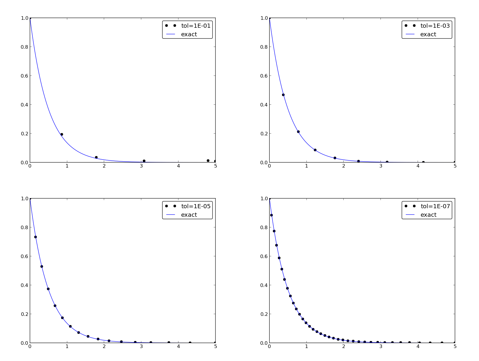
Computing convergence rates
Estimating the convergence rate \( r \)
Implementation
Execution
Debugging via convergence rates
Memory-saving implementation
Memory-saving solver function
Reading computed data from file
Usage of memory-saving code
Software engineering
Making a module
Test block
Prefixing imported functions by the module name
Downside of module prefix notation
Doctests
Running doctests
Unit testing with nose
Basic use of nose
Example on a nose test in the source code
Example on a nose test in a separate file
The habit of writing nose tests
Purpose of a test function: raise AssertionError if failure
Advantages of nose
Demonstrating nose (ideas)
Demonstrating nose (code)
Floats as test results require careful comparison
Test of wrong use
Test of convergence rates
Classical unit testing with unittest
Basic use of unittest
Demonstration of unittest
Implementing simple problem and solver classes
What to learn
The problem class
Improved problem class
The solver class
The visualizer class
Combing the classes
Implementing more advanced problem and solver classes
A generic class for parameters
The problem class
The solver class
The visualizer class
Performing scientific experiments
Model problem and numerical solution method
Plan for the experiments
Typical plot summarizing the results
Script code
Comments to the code
Interpreting output from other programs
Code for grabbing output from another program
Code for interpreting the grabbed output
Making a report
Publishing a complete project
Analysis of finite difference equations
Encouraging numerical solutions
Discouraging numerical solutions; Crank-Nicolson
Discouraging numerical solutions; Forward Euler
Summary of observations
Problem setting
Experimental investigation of oscillatory solutions
Exact numerical solution
Stability
Computation of stability in this problem
Computation of stability in this problem
Explanation of problems with Forward Euler
Explanation of problems with Crank-Nicolson
Summary of stability
Comparing amplification factors
Plot of amplification factors
Series expansion of amplification factors
Error in amplification factors
The fraction of numerical and exact amplification factors
The true/global error at a point
Computing the global error at a point
Convergence
Integrated errors
Truncation error
Computation of the truncation error
The truncation error for other schemes
Consistency, stability, and convergence
Model extensions
Extension to a variable coefficient; Forward and Backward Euler
Extension to a variable coefficient; Crank-Nicolson
Extension to a variable coefficient; \( \theta \)-rule
Extension to a variable coefficient; operator notation
Extension to a source term
Implementation of the generalized model problem
Implementations of variable coefficients; functions
Implementations of variable coefficients; classes
Implementations of variable coefficients; lambda function
Verification via trivial solutions
Verification via trivial solutions; nose test
Verification via manufactured solutions
Linear manufactured solution
Nose test for linear manufactured solution
Extension to systems of ODEs
The Backward Euler method gives a system of algebraic equations
General first-order ODEs
Generic form
The \( \theta \)-rule
Implicit 2-step backward scheme
The Leapfrog scheme
The filtered Leapfrog scheme
2nd-order Runge-Kutta scheme
4th-order Runge-Kutta scheme
2nd-order Adams-Bashforth scheme
3rd-order Adams-Bashforth scheme
The Odespy software
Example: Runge-Kutta methods
Plots from the experiments
Example: Adaptive Runge-Kutta methods
After having completed INF5620 you
numpy, scipy, matplotlib,
sympy, fenics, scitools, ...
What if you don't have this ideal background?
Everything we do is motivated by what we need as building blocks for solving PDEs!
sympy software
for symbolic computation
The world's simplest (?) ODE:
$$ \begin{equation*} u'(t) = -au(t),\quad u(0)=I,\ t\in (0,T]\tp \end{equation*} $$
$$ \begin{equation} u' = -au,\ t\in (0,T], \quad u(0)=I\tp \label{decay:problem} \end{equation} $$
Solution of the continuous problem ("continuous solution"):
$$ \begin{equation*} u(t) = Ie^{-at}\tp\end{equation*} $$ (special case that we can derive a formula for the discrete solution)
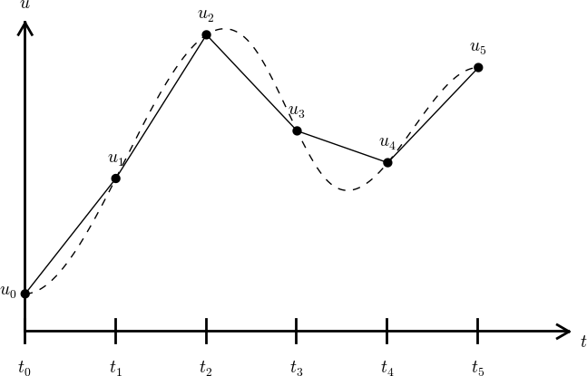
\( u^n\approx u(t_n) \) means that \( u \) is found at discrete time points \( t_1,t_2,t_3,\ldots \)
Typical computational formula: $$ \begin{equation*} u^{n+1} = Au^n\tp\end{equation*} $$ The constant \( A \) depends on the type of finite difference method.
Solution of the discrete problem ("discrete solution"):
$$ \begin{equation*} u^{n+1} = IA^n\tp\end{equation*} $$ (special case that we can derive a formula for the discrete solution)
Solving a differential equation by a finite difference method consists of four steps:
The time domain \( [0,T] \) is represented by a mesh: a finite number of \( N_t+1 \) points
$$0 = t_0 < t_1 < t_2 < \cdots < t_{N_t-1} < t_{N_t} = T\tp$$
\( u^n \) is a mesh function, defined at the mesh points \( t_n \), \( n=0,\ldots,N_t \) only.
Can extend the mesh function to yield values between mesh points by linear interpolation:
$$ \begin{equation} u(t) \approx u^n + \frac{u^{n+1}-u^n}{t_{n+1}-t_n}(t - t_n)\tp \end{equation} $$
Now it is time for the finite difference approximations of derivatives:
$$ \begin{equation} u'(t_n) \approx \frac{u^{n+1}-u^{n}}{t_{n+1}-t_n}\tp \label{decay:FEdiff} \end{equation} $$

Inserting the finite difference approximation in
$$ u'(t_n) = -au(t_n),$$ gives
$$ \begin{equation} \frac{u^{n+1}-u^{n}}{t_{n+1}-t_n} = -au^{n},\quad n=0,1,\ldots,N_t-1\tp \label{decay:step3} \end{equation} $$
This is the
$$ \begin{equation} u^{n+1} = u^n - a(t_{n+1} -t_n)u^n\tp \label{decay:FE} \end{equation} $$
Assume constant time spacing: \( \Delta t = t_{n+1}-t_n=\mbox{const} \)
$$ \begin{align*} u_0 &= I,\\ u_1 & = u^0 - a\Delta t u^0 = I(1-a\Delta t),\\ u_2 & = I(1-a\Delta t)^2,\\ u^3 &= I(1-a\Delta t)^3,\\ &\vdots\\ u^{N_t} &= I(1-a\Delta t)^{N_t}\tp \end{align*} $$
Ooops - we can find the numerical solution by hand (in this simple example)! No need for a computer (yet)...
Here is another finite difference approximation to the derivative (backward difference):
$$ \begin{equation} u'(t_n) \approx \frac{u^{n}-u^{n-1}}{t_{n}-t_{n-1}}\tp \label{decay:BEdiff} \end{equation} $$

Inserting the finite difference approximation in \( u'(t_n)=-au(t_n) \) yields the Backward Euler (BE) scheme:
$$ \begin{equation} \frac{u^{n}-u^{n-1}}{t_{n}-t_{n-1}} = -a u^n\tp \label{decay:BE0} \end{equation} $$ Solve with respect to the unknown \( u^{n+1} \):
$$ \begin{equation} u^{n+1} = \frac{1}{1+ a(t_{n+1}-t_n)} u^n\tp \label{decay:BE} \end{equation} $$
Centered differences are better approximations than forward or backward differences.
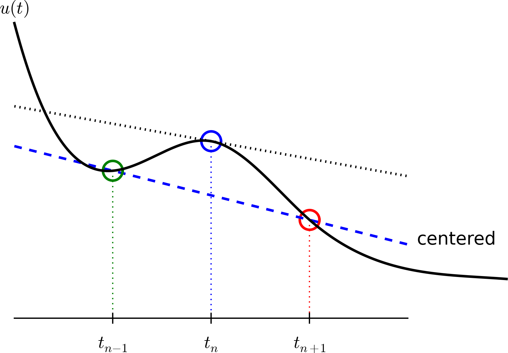
Idea 1: let the ODE hold at \( t_{n+1/2} \)
$$ u'(t_{n+1/2} = -au(t_{n+1/2})\tp$$
Idea 2: approximate \( u'(t_{n+1/2} \) by a centered difference
$$ \begin{equation} u'(t_{n+\half}) \approx \frac{u^{n+1}-u^n}{t_{n+1}-t_n}\tp \label{decay:CNdiff} \end{equation} $$
Problem: \( u(t_{n+1/2}) \) is not defined, only \( u^n=u(t_n) \) and \( u^{n+1}=u(t_{n+1}) \)
Solution:
$$ u(t_{n+1/2}) \approx \half(u^n + u^{n+1}) $$
Result:
$$ \begin{equation} \frac{u^{n+1}-u^n}{t_{n+1}-t_n} = -a\half (u^n + u^{n+1})\tp \label{decay:CN1} \end{equation} $$
Solve wrt to \( u^{n+1} \):
$$ \begin{equation} u^{n+1} = \frac{1-\half a(t_{n+1}-t_n)}{1 + \half a(t_{n+1}-t_n)}u^n\tp \label{decay:CN} \end{equation} $$ This is a Crank-Nicolson (CN) scheme or a midpoint or centered scheme.
The Forward Euler, Backward Euler, and Crank-Nicolson schemes can be formulated as one scheme with a varying parameter \( \theta \):
$$ \begin{equation} \frac{u^{n+1}-u^{n}}{t_{n+1}-t_n} = -a (\theta u^{n+1} + (1-\theta) u^{n}) \label{decay:th0} \tp \end{equation} $$
$$ \begin{equation} u^{n+1} = \frac{1 - (1-\theta) a(t_{n+1}-t_n)}{1 + \theta a(t_{n+1}-t_n)}\tp \label{decay:th} \end{equation} $$
Very common assumption (not important, but exclusively used for simplicity hereafter): constant time step \( t_{n+1}-t_n\equiv\Delta t \)
Derive Forward Euler, Backward Euler, and Crank-Nicolson schemes for Newton's law of cooling:
$$ T' = -k(T-T_s),\quad T(0)=T_0,\ t\in (0,t_{\mbox{end}}]\tp$$
Physical quantities:
Forward difference:
$$ \begin{equation} [D_t^+u]^n = \frac{u^{n+1} - u^{n}}{\Delta t} \approx \frac{d}{dt} u(t_n) \label{fd:D:f} \tp \end{equation} $$ Centered difference:
$$ \begin{equation} [D_tu]^n = \frac{u^{n+\half} - u^{n-\half}}{\Delta t} \approx \frac{d}{dt} u(t_n), \label{fd:D:c} \end{equation} $$
Backward difference: $$ \begin{equation} [D_t^-u]^n = \frac{u^{n} - u^{n-1}}{\Delta t} \approx \frac{d}{dt} u(t_n) \label{fd:D:b} \end{equation} $$
$$ \begin{equation*} [D_t^-u]^n = -au^n \tp \end{equation*} $$
Common to put the whole equation inside square brackets:
$$ \begin{equation} [D_t^- u = -au]^n \tp \end{equation} $$
$$ \begin{equation} [D_t^+ u = -au]^n\tp \end{equation} $$
Introduce an averaging operator:
$$ \begin{equation} [\overline{u}^{t}]^n = \half (u^{n-\half} + u^{n+\half} ) \approx u(t_n) \label{fd:mean:a} \end{equation} $$
The Crank-Nicolson scheme can then be written as
$$ \begin{equation} [D_t u = -a\overline{u}^t]^{n+\half}\tp \label{fd:compact:ex:CN} \end{equation} $$
Test: use the definitions and write out the above formula to see that it really is the Crank-Nicolson scheme!
Model: $$ u'(t) = -au(t),\quad t\in (0,T], \quad u(0)=I, $$
Numerical method:
$$ u^{n+1} = \frac{1 - (1-\theta) a\Delta t}{1 + \theta a\Delta t}u^n, $$ for \( \theta\in [0,1] \). Note
argparse.ArgumentParser
u.
from numpy import *

def solver(I, a, T, dt, theta):
    """Solve u'=-a*u, u(0)=I, for t in (0,T] with steps of dt."""
    Nt = int(T/dt)            # no of time intervals
    T = Nt*dt                 # adjust T to fit time step dt
    u = zeros(Nt+1)           # array of u[n] values
    t = linspace(0, T, Nt+1)  # time mesh

    u[0] = I                  # assign initial condition
    for n in range(0, Nt):    # n=0,1,...,Nt-1
        u[n+1] = (1 - (1-theta)*a*dt)/(1 + theta*dt*a)*u[n]
    return u, t
Note about the for loop: range(0, Nt, s) generates all integers
from 0 to Nt in steps of s (default 1), but not including Nt (!).
Sample call:
u, t = solver(I=1, a=2, T=8, dt=0.8, theta=1)
Python applies integer division: 1/2 is 0, while 1./2 or 1.0/2 or
1/2. or 1/2.0 or 1.0/2.0 all give 0.5.
A safer solver function (dt = float(dt) - guarantee float):
from numpy import *

def solver(I, a, T, dt, theta):
    """Solve u'=-a*u, u(0)=I, for t in (0,T] with steps of dt."""
    dt = float(dt)            # avoid integer division
    Nt = int(round(T/dt))     # no of time intervals
    T = Nt*dt                 # adjust T to fit time step dt
    u = zeros(Nt+1)           # array of u[n] values
    t = linspace(0, T, Nt+1)  # time mesh

    u[0] = I                  # assign initial condition
    for n in range(0, Nt):    # n=0,1,...,Nt-1
        u[n+1] = (1 - (1-theta)*a*dt)/(1 + theta*dt*a)*u[n]
    return u, t
def solver(I, a, T, dt, theta):
    """
    Solve

        u'(t) = -a*u(t),

    with initial condition u(0)=I, for t in the time interval
    (0,T]. The time interval is divided into time steps of
    length dt.

    theta=1 corresponds to the Backward Euler scheme, theta=0
    to the Forward Euler scheme, and theta=0.5 to the Crank-
    Nicolson method.
    """
    ...
Can control formatting of reals and integers through the printf format:
print 't=%6.3f u=%g' % (t[i], u[i])
Or the alternative format string syntax:
print 't={t:6.3f} u={u:g}'.format(t=t[i], u=u[i])
How to run the program decay_v1.py:
Terminal> python decay_v1.py
Can also run it as "normal" Unix programs: ./decay_v1.py if the
first line is
`#!/usr/bin/env python`
Then
Terminal> chmod a+rx decay_v1.py
Terminal> ./decay_v1.py
Use a calculator (\( I=0.1 \), \( \theta=0.8 \), \( \Delta t =0.8 \)):
$$ A\equiv \frac{1 - (1-\theta) a\Delta t}{1 + \theta a \Delta t} = 0.298245614035$$
$$ \begin{align*} u^1 &= AI=0.0298245614035,\\ u^2 &= Au^1= 0.00889504462912,\\ u^3 &=Au^2= 0.00265290804728 \end{align*} $$
See the function verify_three_steps in decay_verf1.py.
Define $$ A = \frac{1 - (1-\theta) a\Delta t}{1 + \theta a \Delta t}\tp $$ Repeated use of the \( \theta \)-rule: $$ \begin{align*} u^0 &= I,\\ u^1 &= Au^0 = AI,\\ u^n &= A^nu^{n-1} = A^nI \tp \end{align*} $$
The exact discrete solution as $$ \begin{equation} u^n = IA^n \label{decay:un:exact} \tp \end{equation} $$
Test if
$$ \max_n |u^n - \uex(t_n)| < \epsilon\sim 10^{-15}$$
Implementation in decay_verf2.py.
Make a program for solving Newton's law of cooling
$$ T' = -k(T-T_s),\quad T(0)=T_0,\ t\in (0,t_{\mbox{end}}]\tp$$ with the Forward Euler, Backward Euler, and Crank-Nicolson schemes (or a \( \theta \) scheme). Verify the implementation.
Task: compute the numerical error \( e^n = \uex(t_n) - u^n \)
Exact solution: \( \uex(t)=Ie^{-at} \), implemented as
def exact_solution(t, I, a):
    return I*exp(-a*t)
Compute \( e^n \) by
u, t = solver(I, a, T, dt, theta)  # Numerical solution
u_e = exact_solution(t, I, a)
e = u_e - u
exact_solution(t, I, a) works with t as arrayexp from numpy (not math)e = u_e - u: array subtraction
$$ \begin{align} ||f||_{L^2} &= \left( \int_0^T f(t)^2 dt\right)^{1/2} \label{decay:norms:L2}\\ ||f||_{L^1} &= \int_0^T |f(t)| dt \label{decay:norms:L1}\\ ||f||_{L^\infty} &= \max_{t\in [0,T]}|f(t)| \label{decay:norms:Linf} \end{align} $$
$$ ||f^n|| = \left(\Delta t\left(\half(f^0)^2 + \half(f^{N_t})^2 + \sum_{n=1}^{N_t-1} (f^n)^2\right)\right)^{1/2} $$
Common simplification yields the \( L^2 \) norm of a mesh function:
$$ ||f^n||_{\ell^2} = \left(\Delta t\sum_{n=0}^{N_t} (f^n)^2\right)^{1/2} \tp$$
$$ E = ||e^n||_{\ell^2} = \sqrt{\Delta t\sum_{n=0}^{N_t} (e^n)^2}$$
Python w/array arithmetics:
e = u_exact(t) - u
E = sqrt(dt*sum(e**2))
Scalar computing of E = sqrt(dt*sum(e**2)):
m = len(u)     # length of u array (alt: u.size)
u_e = zeros(m)
t = 0
for i in range(m):
    u_e[i] = exact_solution(t, a, I)
    t = t + dt
e = zeros(m)
for i in range(m):
    e[i] = u_e[i] - u[i]
s = 0  # summation variable
for i in range(m):
    s = s + e[i]**2
error = sqrt(dt*s)
Obviously, scalar computing
Basic plotting with Matplotlib is much like MATLAB plotting
from matplotlib.pyplot import *
plot(t, u)
show()
Compare u curve with \( \uex(t) \):
t_e = linspace(0, T, 1001)      # fine mesh
u_e = exact_solution(t_e, I, a)
plot(t_e, u_e, 'b-')            # blue line for u_e
plot(t,   u,   'r--o')          # red dashes w/circles
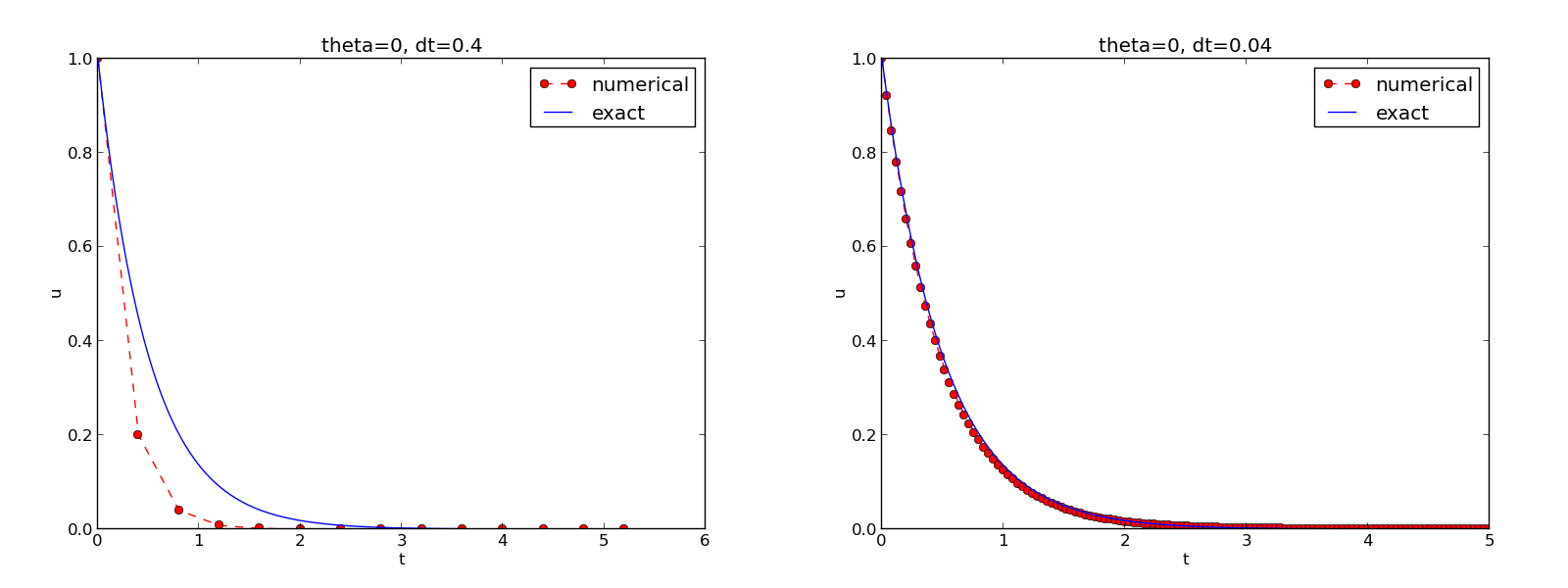
from matplotlib.pyplot import *
figure() # create new plot
t_e = linspace(0, T, 1001) # fine mesh for u_e
u_e = exact_solution(t_e, I, a)
plot(t, u, 'r--o') # red dashes w/circles
plot(t_e, u_e, 'b-') # blue line for exact sol.
legend(['numerical', 'exact'])
xlabel('t')
ylabel('u')
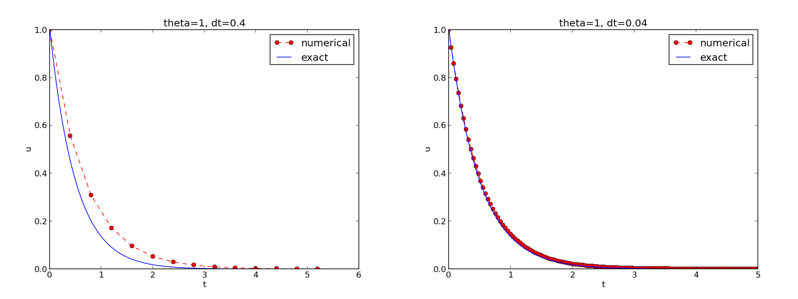
title('theta=%g, dt=%g' % (theta, dt))
savefig('%s_%g.png' % (theta, dt))
show()
See complete code in decay_plot_mpl.py.
SciTools provides a unified plotting interface (Easyviz) to many different plotting packages: Matplotlib, Gnuplot, Grace, VTK, OpenDX, ...
Can use Matplotlib (MATLAB-like) syntax,
or a more compact plot function syntax:
from scitools.std import *

plot(t,   u,   'r--o',           # red dashes w/circles
     t_e, u_e, 'b-',             # blue line for exact sol.
     legend=['numerical', 'exact'],
     xlabel='t',
     ylabel='u',
     title='theta=%g, dt=%g' % (theta, dt),
     savefig='%s_%g.png' % (theta2name[theta], dt),
     show=True)
Complete code in decay_plot_st.py.
Change backend (plotting engine, Matplotlib by default):
Terminal> python decay_plot_st.py --SCITOOLS_easyviz_backend gnuplot
Terminal> python decay_plot_st.py --SCITOOLS_easyviz_backend grace
sys.argvsys.argv[0] is the programsys.argv[1:] holds the command-line arguments--option value pairs on the command line (with default values)
Terminal> python myprog.py 1.5 2 0.5 0.8 0.4
Terminal> python myprog.py --I 1.5 --a 2 --dt 0.8 0.4
The program decay_plot_mpl.py needs this input:
makeplot)
Terminal> python decay_cml.py 1.5 2 0.5 0.8 0.4
import sys

def read_command_line():
    if len(sys.argv) < 6:
        print 'Usage: %s I a T on/off dt1 dt2 dt3 ...' % \
              sys.argv[0]; sys.exit(1)  # abort

    I = float(sys.argv[1])
    a = float(sys.argv[2])
    T = float(sys.argv[3])
    makeplot = sys.argv[4] in ('on', 'True')
    dt_values = [float(arg) for arg in sys.argv[5:]]

    return I, a, T, makeplot, dt_values
Note:
sys.argv[i] is always a stringfloat for computations[expression for e in somelist]
Set option-value pairs on the command line if the default value is not suitable:
Terminal> python decay_argparse.py --I 1.5 --a 2 --dt 0.8 0.4
Code:
def define_command_line_options():
    import argparse
    parser = argparse.ArgumentParser()
    parser.add_argument('--I', '--initial_condition', type=float,
                        default=1.0, help='initial condition, u(0)',
                        metavar='I')
    parser.add_argument('--a', type=float,
                        default=1.0, help='coefficient in ODE',
                        metavar='a')
    parser.add_argument('--T', '--stop_time', type=float,
                        default=1.0, help='end time of simulation',
                        metavar='T')
    parser.add_argument('--makeplot', action='store_true',
                        help='display plot or not')
    parser.add_argument('--dt', '--time_step_values', type=float,
                        default=[1.0], help='time step values',
                        metavar='dt', nargs='+', dest='dt_values')
    return parser
(metavar is the symbol used in help output)
argparse.ArgumentParser parses the command-line arguments:
def read_command_line():
    parser = define_command_line_options()
    args = parser.parse_args()
    print 'I={}, a={}, T={}, makeplot={}, dt_values={}'.format(
        args.I, args.a, args.T, args.makeplot, args.dt_values)
    return args.I, args.a, args.T, args.makeplot, args.dt_values
Complete program: decay_argparse.py.
Normally very much programming required - and much competence on graphical user interfaces.
Here: use a tool to automatically create it in a few minutes (!)
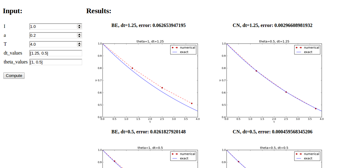
main function carries out simulations and plotting for a
series of \( \Delta t \) valuesparampool functionalitymain_GUI:
def main_GUI(I=1.0, a=.2, T=4.0,
         dt_values=[1.25, 0.75, 0.5, 0.1],
         theta_values=[0, 0.5, 1]):
explore solves the problem, makes a plot, computes the
error and returns appropriate HTML code with the plot. Embed
error and plots in a table:
def main_GUI(I=1.0, a=.2, T=4.0,
         dt_values=[1.25, 0.75, 0.5, 0.1],
         theta_values=[0, 0.5, 1]):
    # Build HTML code for web page. Arrange plots in columns
    # corresponding to the theta values, with dt down the rows
    theta2name = {0: 'FE', 1: 'BE', 0.5: 'CN'}
    html_text = '<table>\n'
    for dt in dt_values:
        html_text += '<tr>\n'
        for theta in theta_values:
            E, html = explore(I, a, T, dt, theta, makeplot=True)
            html_text += """
<td>
<center><b>%s, dt=%g, error: %s</b></center><br>
%s
</td>
""" % (theta2name[theta], dt, E, html)
        html_text += '</tr>\n'
    html_text += '</table>\n'
    return html_text
In explore:
import matplotlib.pyplot as plt
...
# plot
plt.plot(t, u, r-')
plt.xlabel('t')
plt.ylabel('u')
...
from parampool.utils import save_png_to_str
html_text = save_png_to_str(plt, plotwidth=400)
If you know HTML, you can return more sophisticated layout etc.
Make a file decay_GUI_generate.py:
from parampool.generator.flask import generate
from decay_GUI import main
generate(main,
         output_controller='decay_GUI_controller.py',
         output_template='decay_GUI_view.py',
         output_model='decay_GUI_model.py')
Running decay_GUI_generate.py results in
decay_GUI_model.py defines HTML widgets to be used to set
input data in the web interface,templates/decay_GUI_views.py defines the layout of the web page,decay_GUI_controller.py runs the web application.decay_GUI_controller.py
and there is no need to look into any of these files!
Start the GUI
Terminal> python decay_GUI_controller.py
Open a web browser at 127.0.0.1:5000
Frequent assumption on the relation between the numerical error \( E \) and some discretization parameter \( \Delta t \):
$$ \begin{equation} E = C\Delta t^r, \label{decay:E:dt} \end{equation} $$
Perform numerical experiments: \( (\Delta t_i, E_i) \), \( i=0,\ldots,m-1 \). Two methods for finding \( r \) (and \( C \)):
Method 2 is best.
Compute \( r_0, r_1, \ldots, r_{m-2} \):
from math import log

def main():
    I, a, T, makeplot, dt_values = read_command_line()
    r = {}  # estimated convergence rates
    for theta in 0, 0.5, 1:
        E_values = []
        for dt in dt_values:
            E = explore(I, a, T, dt, theta, makeplot=False)
            E_values.append(E)

        # Compute convergence rates
        m = len(dt_values)
        r[theta] = [log(E_values[i-1]/E_values[i])/
                    log(dt_values[i-1]/dt_values[i])
                    for i in range(1, m, 1)]

    for theta in r:
        print '\nPairwise convergence rates for theta=%g:' % theta
        print ' '.join(['%.2f' % r_ for r_ in r[theta]])
    return r
Complete program: decay_convrate.py.
Terminal> python decay_convrate.py --dt 0.5 0.25 0.1 0.05 0.025 0.01
...
Pairwise convergence rates for theta=0:
1.33 1.15 1.07 1.03 1.02

Pairwise convergence rates for theta=0.5:
2.14 2.07 2.03 2.01 2.01

Pairwise convergence rates for theta=1:
0.98 0.99 0.99 1.00 1.00
Potential bug: missing a in the denominator,
u[n+1] = (1 - (1-theta)*a*dt)/(1 + theta*dt)*u[n]
Running decay_convrate.py gives same rates.
Why? The value of \( a \)... (\( a=1 \))
0 and 1 are bad values in tests!
Better:
Terminal> python decay_convrate.py --a 2.1 --I 0.1  \
          --dt 0.5 0.25 0.1 0.05 0.025 0.01
...
Pairwise convergence rates for theta=0:
1.49 1.18 1.07 1.04 1.02

Pairwise convergence rates for theta=0.5:
-1.42 -0.22 -0.07 -0.03 -0.01

Pairwise convergence rates for theta=1:
0.21 0.12 0.06 0.03 0.01
Forward Euler works...because \( \theta=0 \) hides the bug.
This bug gives \( r\approx 0 \):
u[n+1] = ((1-theta)*a*dt)/(1 + theta*dt*a)*u[n]
u, i.e., \( u^n \) for \( n=0,1,\ldots,N_t \)u, \( u^n \) in u_1 (float)u in a file, read file later for plotting
def solver_memsave(I, a, T, dt, theta, filename='sol.dat'):
    """
    Solve u'=-a*u, u(0)=I, for t in (0,T] with steps of dt.
    Minimum use of memory. The solution is stored in a file
    (with name filename) for later plotting.
    """
    dt = float(dt)         # avoid integer division
    Nt = int(round(T/dt))  # no of intervals

    outfile = open(filename, 'w')
    # u: time level n+1, u_1: time level n
    t = 0
    u_1 = I
    outfile.write('%.16E  %.16E\n' % (t, u_1))
    for n in range(1, Nt+1):
        u = (1 - (1-theta)*a*dt)/(1 + theta*dt*a)*u_1
        u_1 = u
        t += dt
        outfile.write('%.16E  %.16E\n' % (t, u))
    outfile.close()
    return u, t
def read_file(filename='sol.dat'):
    infile = open(filename, 'r')
    u = [];  t = []
    for line in infile:
        words = line.split()
        if len(words) != 2:
            print 'Found more than two numbers on a line!', words
            sys.exit(1)  # abort
        t.append(float(words[0]))
        u.append(float(words[1]))
    return np.array(t), np.array(u)
Simpler code with numpy functionality for reading/writing tabular data:
def read_file_numpy(filename='sol.dat'):
    data = np.loadtxt(filename)
    t = data[:,0]
    u = data[:,1]
    return t, u
Similar function np.savetxt, but then we need all \( u^n \) and \( t^n \) values
in a two-dimensional array (which we try to prevent now!).
def explore(I, a, T, dt, theta=0.5, makeplot=True):
    filename = 'u.dat'
    u, t = solver_memsave(I, a, T, dt, theta, filename)

    t, u = read_file(filename)
    u_e = exact_solution(t, I, a)
    e = u_e - u
    E = np.sqrt(dt*np.sum(e**2))
    if makeplot:
        plt.figure()
        ...
Complete program: decay_memsave.py.
Goal: make more professional numerical software.
Topics:
solver)import)solververify_three_stepsverify_discrete_solutionexploredefine_command_line_optionsread_command_linemain (with convergence rates)verify_convergence_ratedecay_mod, filename: decay_mod.py.
Sketch:
from numpy import *
from matplotlib.pyplot import *
import sys

def solver(I, a, T, dt, theta):
    ...

def verify_three_steps():
    ...

def verify_exact_discrete_solution():
    ...

def exact_solution(t, I, a):
    ...

def explore(I, a, T, dt, theta=0.5, makeplot=True):
    ...

def define_command_line_options():
    ...

def read_command_line(use_argparse=True):
    ...

def main():
    ...
That is! It's a module decay_mod in file decay_mod.py.
Usage in some other program:
from decay_mod import solver
u, t = solver(I=1.0, a=3.0, T=3, dt=0.01, theta=0.5)
At the end of a module it is common to include a test block:
if __name__ == '__main__':
    main()
decay_mod is imported, __name__ is decay_mod.decay_mod.py is run, __name__ is __main__.
if __name__ == '__main__':
    if 'verify' in sys.argv:
        if verify_three_steps() and verify_discrete_solution():
            pass # ok
        else:
            print 'Bug in the implementation!'
    elif 'verify_rates' in sys.argv:
        sys.argv.remove('verify_rates')
        if not '--dt' in sys.argv:
            print 'Must assign several dt values'
            sys.exit(1)  # abort
        if verify_convergence_rate():
            pass
        else:
            print 'Bug in the implementation!'
    else:
        # Perform simulations
        main()
from numpy import *
from matplotlib.pyplot import *
This imports a large number of names (sin, exp, linspace, plot, ...).
Confusion: is a function from`numpy`? Or matplotlib.pyplot?
Alternative (recommended) import:
import numpy
import matplotlib.pyplot
Now we need to prefix functions with module name:
t = numpy.linspace(0, T, Nt+1)
u_e = I*numpy.exp(-a*t)
matplotlib.pyplot.plot(t, u_e)
Common standard:
import numpy as np
import matplotlib.pyplot as plt

t = np.linspace(0, T, Nt+1)
u_e = I*np.exp(-a*t)
plt.plot(t, u_e)
A math line like \( e^{-at}\sin(2\pi t) \) gets cluttered with module names,
numpy.exp(-a*t)*numpy.sin(2(numpy.pi*t)
# or
np.exp(-a*t)*np.sin(2*np.pi*t)
Solution (much used in this course): do two imports
import numpy as np
from numpy import exp, sin, pi
...
t = np.linspace(0, T, Nt+1)
u_e = exp(-a*t)*sin(2*pi*t)
Doc strings can be equipped with interactive Python sessions for demonstrating usage and automatic testing of functions.
def solver(I, a, T, dt, theta):
    """
    Solve u'=-a*u, u(0)=I, for t in (0,T] with steps of dt.


    >>> u, t = solver(I=0.8, a=1.2, T=4, dt=0.5, theta=0.5)
    >>> for t_n, u_n in zip(t, u):
    ...     print 't=%.1f, u=%.14f' % (t_n, u_n)
    t=0.0, u=0.80000000000000
    t=0.5, u=0.43076923076923
    t=1.0, u=0.23195266272189
    t=1.5, u=0.12489758761948
    t=2.0, u=0.06725254717972
    t=2.5, u=0.03621291001985
    t=3.0, u=0.01949925924146
    t=3.5, u=0.01049960113002
    t=4.0, u=0.00565363137770
    """
    ...
Automatic check that the code reproduces the doctest output:
Terminal> python -m doctest decay_mod_doctest.py
Report in case of failure:
Terminal> python -m doctest decay_mod_doctest.py
********************************************************
File "decay_mod_doctest.py", line 12, in decay_mod_doctest....
Failed example:
    for t_n, u_n in zip(t, u):
        print 't=%.1f, u=%.14f' % (t_n, u_n)
Expected:
    t=0.0, u=0.80000000000000
    t=0.5, u=0.43076923076923
    t=1.0, u=0.23195266272189
    t=1.5, u=0.12489758761948
    t=2.0, u=0.06725254717972
Got:
    t=0.0, u=0.80000000000000
    t=0.5, u=0.43076923076923
    t=1.0, u=0.23195266272189
    t=1.5, u=0.12489758761948
    t=2.0, u=0.06725254718756
********************************************************
1 items had failures:
   1 of   2 in decay_mod_doctest.solver
***Test Failed*** 1 failures.
Complete program: decay_mod_doctest.py.
test_.assert functions from the nose.tools module.test*.py.
Very simple module mymod (in file mymod.py):
def double(n):
    return 2*n
Write test function in mymod.py:
def double(n):
    return 2*n

import nose.tools as nt

def test_double():
    result = double(4)
    nt.assert_equal(result, 8)
Running
Terminal> nosetests -s mymod
makes the nose tool run all test_*() functions in mymod.py.
Write the test in a separate file, say test_mymod.py:
import nose.tools as nt
import mymod

def test_double():
    result = mymod.double(4)
    nt.assert_equal(result, 8)
Running
Terminal> nosetests -s
makes the nose tool run all test_*() functions in all files
test*.py in the current directory and in all subdirectories (recursevely)
with names tests or *_tests.
test_*() functions in the moduletest_*() functions, collect them in
tests/test*.py
Alternative ways of raising AssertionError if result is not 8:
import nose.tools as nt

def test_double():
    result = ...

    nt.assert_equal(result, 8)    # alternative 1

    assert result == 8            # alternative 2

    if result != 8:               # alternative 3
        raise AssertionError()
nosetests -s)
Aim: test function solver for \( u'=-au \), \( u(0)=I \).
We design three unit tests:
verify* functions.
import nose.tools as nt
import decay_mod_unittest as decay_mod
import numpy as np

def exact_discrete_solution(n, I, a, theta, dt):
    """Return exact discrete solution of the theta scheme."""
    dt = float(dt)  # avoid integer division
    factor = (1 - (1-theta)*a*dt)/(1 + theta*dt*a)
    return I*factor**n

def test_exact_discrete_solution():
    """
    Compare result from solver against
    formula for the discrete solution.
    """
    theta = 0.8; a = 2; I = 0.1; dt = 0.8
    N = int(8/dt)  # no of steps
    u, t = decay_mod.solver(I=I, a=a, T=N*dt, dt=dt, theta=theta)
    u_de = np.array([exact_discrete_solution(n, I, a, theta, dt)
                     for n in range(N+1)])
    diff = np.abs(u_de - u).max()
    nt.assert_almost_equal(diff, 0, delta=1E-14)
nt.assert_almost_equal: compare two floats to some digits
or precision
def test_solver():
    """
    Compare result from solver against
    precomputed arrays for theta=0, 0.5, 1.
    """
    I=0.8; a=1.2; T=4; dt=0.5  # fixed parameters
    precomputed = {
        't': np.array([ 0. ,  0.5,  1. ,  1.5,  2. ,  2.5,
                        3. ,  3.5,  4. ]),
        0.5: np.array(
            [ 0.8       ,  0.43076923,  0.23195266, 0.12489759,
              0.06725255,  0.03621291,  0.01949926, 0.0104996 ,
              0.00565363]),
        0: ...,
        1: ...
        }
    for theta in 0, 0.5, 1:
        u, t = decay_mod.solver(I, a, T, dt, theta=theta)
        diff = np.abs(u - precomputed[theta]).max()
        # Precomputed numbers are known to 8 decimal places
        nt.assert_almost_equal(diff, 0, places=8,
                               msg='theta=%s' % theta)
theta = 1; a = 1; I = 1; dt = 2
may lead to integer division:
(1 - (1-theta)*a*dt)  # becomes 1
(1 + theta*dt*a)      # becomes 2
(1 - (1-theta)*a*dt)/(1 + theta*dt*a)  # becomes 0 (!)
Test that solver does not suffer from such integer division:
def test_potential_integer_division():
    """Choose variables that can trigger integer division."""
    theta = 1; a = 1; I = 1; dt = 2
    N = 4
    u, t = decay_mod.solver(I=I, a=a, T=N*dt, dt=dt, theta=theta)
    u_de = np.array([exact_discrete_solution(n, I, a, theta, dt)
                     for n in range(N+1)])
    diff = np.abs(u_de - u).max()
    nt.assert_almost_equal(diff, 0, delta=1E-14)
Convergence rate tests are very common for differential equation solvers.
def test_convergence_rates():
    """Compare empirical convergence rates to exact ones."""
    # Set command-line arguments directly in sys.argv
    import sys
    sys.argv[1:] = '--I 0.8 --a 2.1 --T 5 '\
                   '--dt 0.4 0.2 0.1 0.05 0.025'.split()
    r = decay_mod.main()
    for theta in r:
        nt.assert_true(r[theta])  # check for non-empty list

    expected_rates = {0: 1, 1: 1, 0.5: 2}
    for theta in r:
        r_final = r[theta][-1]
        # Compare to 1 decimal place
        nt.assert_almost_equal(expected_rates[theta], r_final,
                               places=1, msg='theta=%s' % theta)
Complete program: test_decay_nose.py.
unittest is a Python module mimicing the classical JUnit
class-based unit testing framework from Java
Write file test_mymod.py:
import unittest
import mymod

class TestMyCode(unittest.TestCase):
    def test_double(self):
        result = mymod.double(4)
        self.assertEqual(result, 8)

if __name__ == '__main__':
    unittest.main()
import unittest
import decay_mod_unittest as decay
import numpy as np

def exact_discrete_solution(n, I, a, theta, dt):
    factor = (1 - (1-theta)*a*dt)/(1 + theta*dt*a)
    return I*factor**n

class TestDecay(unittest.TestCase):

    def test_exact_discrete_solution(self):
        ...
        diff = np.abs(u_de - u).max()
        self.assertAlmostEqual(diff, 0, delta=1E-14)

    def test_solver(self):
        ...
        for theta in 0, 0.5, 1:
            ...
            self.assertAlmostEqual(diff, 0, places=8,
                                   msg='theta=%s' % theta)

    def test_potential_integer_division():
        ...
        self.assertAlmostEqual(diff, 0, delta=1E-14)

    def test_convergence_rates(self):
        ...
        for theta in r:
            ...
            self.assertAlmostEqual(...)

if __name__ == '__main__':
    unittest.main()
Complete program: test_decay_unittest.py.
Tasks:
Problem stores the physical parameters \( a \), \( I \), \( T \)
from numpy import exp

class Problem:
    def __init__(self, I=1, a=1, T=10):
        self.T, self.I, self.a = I, float(a), T

    def exact_solution(self, t):
        I, a = self.I, self.a     # extract local variables
        return I*exp(-a*t)
Basic usage:
problem = Problem(T=5)
problem.T = 8
problem.dt = 1.5
More flexible input from the command line:
class Problem:
    def __init__(self, I=1, a=1, T=10):
        self.T, self.I, self.a = I, float(a), T

    def define_command_line_options(self, parser=None):
        if parser is None:
            import argparse
            parser = argparse.ArgumentParser()

        parser.add_argument(
            '--I', '--initial_condition', type=float,
            default=self.I, help='initial condition, u(0)',
            metavar='I')
        parser.add_argument(
            '--a', type=float, default=self.a,
            help='coefficient in ODE', metavar='a')
        parser.add_argument(
            '--T', '--stop_time', type=float, default=self.T,
            help='end time of simulation', metavar='T')
        return parser

    def init_from_command_line(self, args):
        self.I, self.a, self.T = args.I, args.a, args.T

    def exact_solution(self, t):
        I, a = self.I, self.a
        return I*exp(-a*t)
ArgumentParser, or make oneNone is used to indicate a non-initialized variable
class Solver:
    def __init__(self, problem, dt=0.1, theta=0.5):
        self.problem = problem
        self.dt, self.theta = float(dt), theta

    def define_command_line_options(self, parser):
        parser.add_argument(
            '--dt', '--time_step_value', type=float,
            default=0.5, help='time step value', metavar='dt')
        parser.add_argument(
            '--theta', type=float, default=0.5,
            help='time discretization parameter', metavar='dt')
        return parser

    def init_from_command_line(self, args):
        self.dt, self.theta = args.dt, args.theta

    def solve(self):
        from decay_mod import solver
        self.u, self.t = solver(
            self.problem.I, self.problem.a, self.problem.T,
            self.dt, self.theta)
Note: reuse of the numerical algorithm from the decay_mod module
(i.e., the class is a wrapper of the procedural implementation).
class Visualizer:
    def __init__(self, problem, solver):
        self.problem, self.solver = problem, solver

    def plot(self, include_exact=True, plt=None):
        """
        Add solver.u curve to the plotting object plt,
        and include the exact solution if include_exact is True.
        This plot function can be called several times (if
        the solver object has computed new solutions).
        """
        if plt is None:
            import scitools.std  as plt # can use matplotlib as well

        plt.plot(self.solver.t, self.solver.u, '--o')
        plt.hold('on')
        theta2name = {0: 'FE', 1: 'BE', 0.5: 'CN'}
        name = theta2name.get(self.solver.theta, '')
        legends = ['numerical %s' % name]
        if include_exact:
            t_e = linspace(0, self.problem.T, 1001)
            u_e = self.problem.exact_solution(t_e)
            plt.plot(t_e, u_e, 'b-')
            legends.append('exact')
        plt.legend(legends)
        plt.xlabel('t')
        plt.ylabel('u')
        plt.title('theta=%g, dt=%g' %
                  (self.solver.theta, self.solver.dt))
        plt.savefig('%s_%g.png' % (name, self.solver.dt))
        return plt
Remark: The plt object in plot adds a new curve to a plot,
which enables comparing different solutions from different
runs of Solver.solve
Let Problem, Solver, and Visualizer play together:
def main():
    problem = Problem()
    solver = Solver(problem)
    viz = Visualizer(problem, solver)

    # Read input from the command line
    parser = problem.define_command_line_options()
    parser = solver. define_command_line_options(parser)
    args = parser.parse_args()
    problem.init_from_command_line(args)
    solver. init_from_command_line(args)

    # Solve and plot
    solver.solve()
    import matplotlib.pyplot as plt
    #import scitools.std as plt
    plt = viz.plot(plt=plt)
    E = solver.error()
    if E is not None:
        print 'Error: %.4E' % E
    plt.show()
Complete program: decay_class.py.
Problem and Solver classes soon contain
much repetitive code when the number of parameters increasesself.prms,
with two associated dictionaries self.types and
self.help for holding associated object types and help stringsParametersProblem, Solver, and maybe Visualizer be subclasses
of class Parameters, basically defining self.prms, self.types,
self.help
class Parameters:
    def set(self, **parameters):
        for name in parameters:
            self.prms[name] = parameters[name]

    def get(self, name):
        return self.prms[name]

    def define_command_line_options(self, parser=None):
        if parser is None:
            import argparse
            parser = argparse.ArgumentParser()

        for name in self.prms:
            tp = self.types[name] if name in self.types else str
            help = self.help[name] if name in self.help else None
            parser.add_argument(
                '--' + name, default=self.get(name), metavar=name,
                type=tp, help=help)

        return parser

    def init_from_command_line(self, args):
        for name in self.prms:
            self.prms[name] = getattr(args, name)
Slightly more advanced version in class_decay_verf1.py.
class Problem(Parameters):
    """
    Physical parameters for the problem u'=-a*u, u(0)=I,
    with t in [0,T].
    """
    def __init__(self):
        self.prms = dict(I=1, a=1, T=10)
        self.types = dict(I=float, a=float, T=float)
        self.help = dict(I='initial condition, u(0)',
                         a='coefficient in ODE',
                         T='end time of simulation')

    def exact_solution(self, t):
        I, a = self.get('I'), self.get('a')
        return I*np.exp(-a*t)
class Solver(Parameters):
    def __init__(self, problem):
        self.problem = problem
        self.prms = dict(dt=0.5, theta=0.5)
        self.types = dict(dt=float, theta=float)
        self.help = dict(dt='time step value',
                         theta='time discretization parameter')

    def solve(self):
        from decay_mod import solver
        self.u, self.t = solver(
            self.problem.get('I'),
            self.problem.get('a'),
            self.problem.get('T'),
            self.get('dt'),
            self.get('theta'))

    def error(self):
        try:
            u_e = self.problem.exact_solution(self.t)
            e = u_e - self.u
            E = np.sqrt(self.get('dt')*np.sum(e**2))
        except AttributeError:
            E = None
        return E
ParametersVisualizerProblem, Solver, and
VisualizerGoal: explore the behavior of a numerical method for a differential equation and show how scientific experiments can be set up and reported.
Tasks:
os.system for running other programssubprocess for running other programs and extracting the outputProblem:
$$ \begin{equation} u'(t) = -au(t),\quad u(0)=I,\ 0< t \leq T, \label{decay:experiments:model} \end{equation} $$
Solution method (\( \theta \)-rule):
$$ u^{n+1} = \frac{1 - (1-\theta) a\Delta t}{1 + \theta a\Delta t}u^n, \quad u^0=I\tp $$
python decay_mod.py --I 1 --a 2 --makeplot --T 5 --dt 0.5 0.25 0.1 0.05FE_*.png, BE_*.png, and CN_*.png
to new figures with multiple plotspython decay_exper0.py 0.5 0.25 0.1 0.05 (\( \Delta t \) values on the command line)

Typical script (small administering program) for running the experiments:
import os, sys

def run_experiments(I=1, a=2, T=5):
    # The command line must contain dt values
    if len(sys.argv) > 1:
        dt_values = [float(arg) for arg in sys.argv[1:]]
    else:
        print 'Usage: %s dt1 dt2 dt3 ...' %  sys.argv[0]
        sys.exit(1)  # abort

    # Run module file as a stand-alone application
    cmd = 'python decay_mod.py --I %g --a %g --makeplot --T %g' % \
          (I, a, T)
    dt_values_str = ' '.join([str(v) for v in dt_values])
    cmd += ' --dt %s' % dt_values_str
    print cmd
    failure = os.system(cmd)
    if failure:
        print 'Command failed:', cmd; sys.exit(1)

    # Combine images into rows with 2 plots in each row
    image_commands = []
    for method in 'BE', 'CN', 'FE':
        pdf_files = ' '.join(['%s_%g.pdf' % (method, dt)
                              for dt in dt_values])
        png_files = ' '.join(['%s_%g.png' % (method, dt)
                              for dt in dt_values])
        image_commands.append(
            'montage -background white -geometry 100%' +
            ' -tile 2x %s %s.png' % (png_files, method))
        image_commands.append(
            'convert -trim %s.png %s.png' % (method, method))
        image_commands.append(
            'convert %s.png -transparent white %s.png' %
            (method, method))
        image_commands.append(
            'pdftk %s output tmp.pdf' % pdf_files)
        num_rows = int(round(len(dt_values)/2.0))
        image_commands.append(
            'pdfnup --nup 2x%d tmp.pdf' % num_rows)
        image_commands.append(
            'pdfcrop tmp-nup.pdf %s.pdf' % method)

    for cmd in image_commands:
        print cmd
        failure = os.system(cmd)
        if failure:
            print 'Command failed:', cmd; sys.exit(1)

    # Remove the files generated above and by decay_mod.py
    from glob import glob
    filenames = glob('*_*.png') + glob('*_*.pdf') + \
                glob('*_*.eps') + glob('tmp*.pdf')
    for filename in filenames:
        os.remove(filename)

if __name__ == '__main__':
    run_experiments()
Complete program: experiments/decay_exper0.py.
Many useful constructs in the previous script:
[float(arg) for arg in sys.argv[1:]] builds a list of real numbers
from all the command-line argumentsfailure = os.system(cmd) runs an operating system command
(e.g., another program)sys.exit(1) aborts the program['%s_%s.png' % (method, dt) for dt in dt_values] builds a list of
filenames from a list of numbers (dt_values)montage commands for creating composite figures are stored in a
list and thereafter executed in a loopglob.glob('*_*.png') returns a list of the names of all files in the
current folder where the filename matches the Unix wildcard notation
*_*.png (meaning "any text, underscore, any text, and then `.png`")os.remove(filename) removes the file with name filename
In decay_exper0.py we run a program (os.system) and
want to grab the output, e.g.,
Terminal> python decay_plot_mpl.py
0.0   0.40:    2.105E-01
0.0   0.04:    1.449E-02
0.5   0.40:    3.362E-02
0.5   0.04:    1.887E-04
1.0   0.40:    1.030E-01
1.0   0.04:    1.382E-02
Tasks:
decay_mod.py program
Use the subprocess module to grab output:
    from subprocess import Popen, PIPE, STDOUT
    p = Popen(cmd, shell=True, stdout=PIPE, stderr=STDOUT)
    output, dummy = p.communicate()
    failure = p.returncode
    if failure:
        print 'Command failed:', cmd; sys.exit(1)
output string, line by lineerrors with keys dt and
the three \( \theta \) values
errors = {'dt': dt_values, 1: [], 0: [], 0.5: []}
for line in output.splitlines():
    words = line.split()
    if words[0] in ('0.0', '0.5', '1.0'):  # line with E?
        # typical line: 0.0   1.25:    7.463E+00
        theta = float(words[0])
        E = float(words[2])
        errors[theta].append(E)
Next: plot \( E \) versus \( \Delta t \) for \( \theta=0,0.5,1 \)
Complete program: experiments/decay_exper1.py. Fine recipe for
Model: $$ \begin{equation} u'(t) = -au(t),\quad u(0)=I, \end{equation} $$
Method: $$ \begin{equation} u^{n+1} = \frac{1 - (1-\theta) a\Delta t}{1 + \theta a\Delta t}u^n \label{decay:analysis:scheme} \end{equation} $$
\( I=1 \), \( a=2 \), \( \theta =1,0.5, 0 \), \( \Delta t=1.25, 0.75, 0.5, 0.1 \).
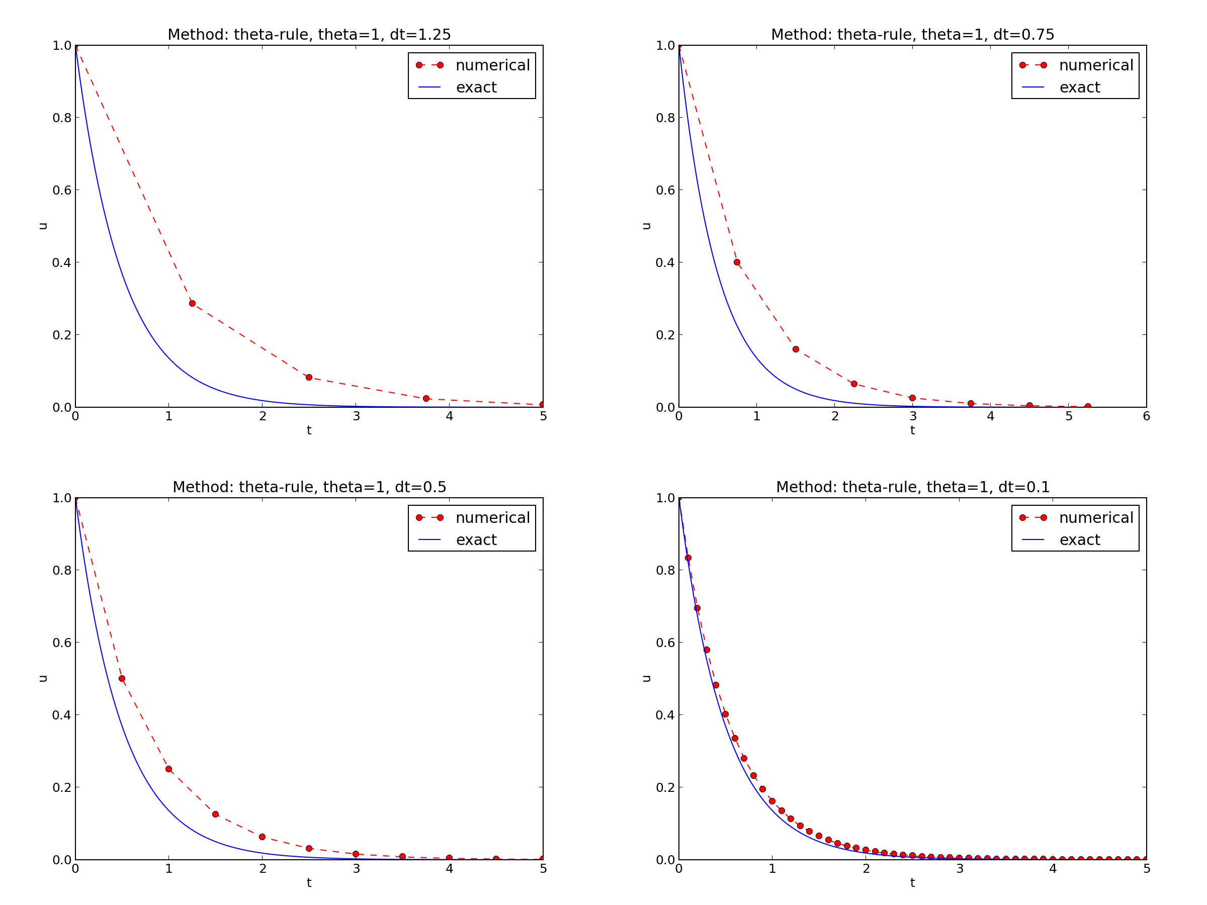
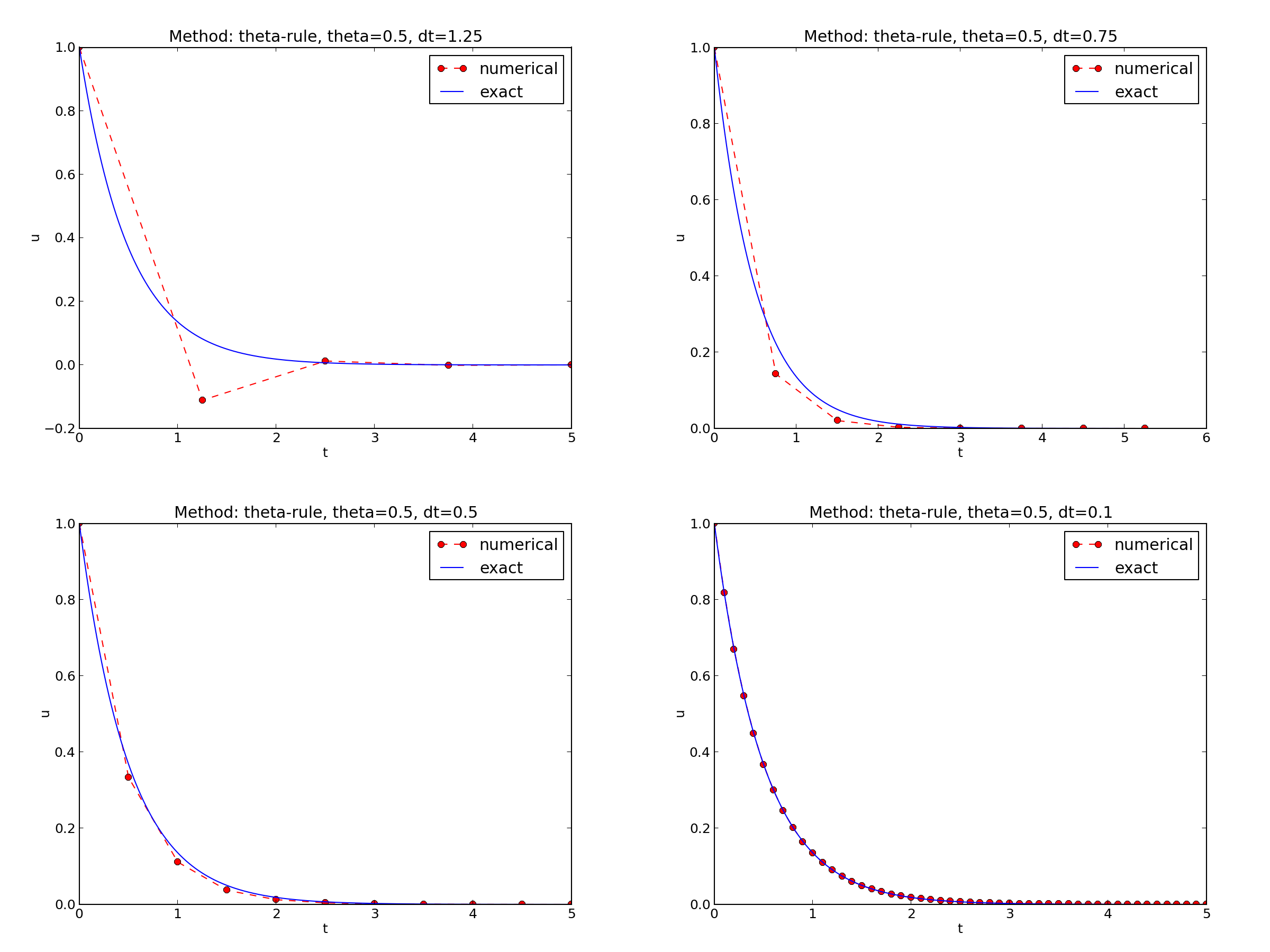

The characteristics of the displayed curves can be summarized as follows:
The solution is oscillatory if $$ u^{n} > u^{n-1},$$
Seems that \( a\Delta t < 1 \) for FE and 2 for CN.
Starting with \( u^0=I \), the simple recursion \eqref{decay:analysis:scheme} can be applied repeatedly \( n \) times, with the result that
$$ \begin{equation} u^{n} = IA^n,\quad A = \frac{1 - (1-\theta) a\Delta t}{1 + \theta a\Delta t}\tp \label{decay:analysis:unex} \end{equation} $$
Such an exact discrete solution is unusual, but very handy for analysis.
Since \( u^n\sim A^n \),
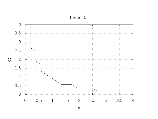
\( A<0 \) if
$$ \frac{1 - (1-\theta) a\Delta t}{1 + \theta a\Delta t} < 0 $$ To avoid oscillatory solutions we must have \( A> 0 \) and
$$ \begin{equation} \Delta t < \frac{1}{(1-\theta)a}\tp \end{equation} $$
\( |A|\leq 1 \) means \( -1\leq A\leq 1 \)
$$ \begin{equation} -1\leq\frac{1 - (1-\theta) a\Delta t}{1 + \theta a\Delta t} \leq 1\tp \label{decay:th:stability} \end{equation} $$ \( -1 \) is the critical limit:
$$ \begin{align*} \Delta t &\leq \frac{2}{(1-2\theta)a},\quad \theta < \half\\ \Delta t &\geq \frac{2}{(1-2\theta)a},\quad \theta > {\half} \end{align*} $$
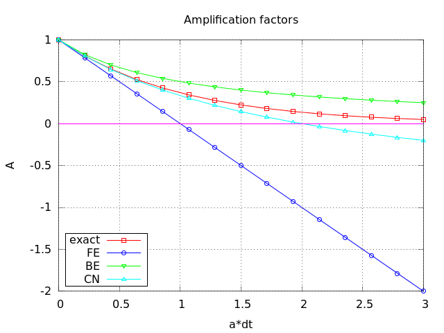
\( u^{n+1} \) is an amplification \( A \) of \( u^n \):
$$ u^{n+1} = Au^n,\quad A = \frac{1 - (1-\theta) a\Delta t}{1 + \theta a\Delta t} $$
The exact solution is also an amplification:
$$ u(t_{n+1}) = \Aex u(t_n), \quad \Aex = e^{-a\Delta t}$$
A possible measure of accuracy: \( \Aex - A \)
To investigate \( \Aex - A \) mathematically, we can Taylor expand the expression, using \( p=a\Delta t \) as variable.
>>> from sympy import *
>>> # Create p as a mathematical symbol with name 'p'
>>> p = Symbol('p')
>>> # Create a mathematical expression with p
>>> A_e = exp(-p)
>>>
>>> # Find the first 6 terms of the Taylor series of A_e
>>> A_e.series(p, 0, 6)
1 + (1/2)*p**2 - p - 1/6*p**3 - 1/120*p**5 + (1/24)*p**4 + O(p**6)

>>> theta = Symbol('theta')
>>> A = (1-(1-theta)*p)/(1+theta*p)
>>> FE = A_e.series(p, 0, 4) - A.subs(theta, 0).series(p, 0, 4)
>>> BE = A_e.series(p, 0, 4) - A.subs(theta, 1).series(p, 0, 4)
>>> half = Rational(1,2)  # exact fraction 1/2
>>> CN = A_e.series(p, 0, 4) - A.subs(theta, half).series(p, 0, 4)
>>> FE
(1/2)*p**2 - 1/6*p**3 + O(p**4)
>>> BE
-1/2*p**2 + (5/6)*p**3 + O(p**4)
>>> CN
(1/12)*p**3 + O(p**4)
Focus: the error measure \( A-\Aex \) as function of \( \Delta t \) (recall that \( p=a\Delta t \)):
$$ \begin{equation} A-\Aex = \left\lbrace\begin{array}{ll} \Oof{\Delta t^2}, & \hbox{Forward and Backward Euler},\\ \Oof{\Delta t^3}, & \hbox{Crank-Nicolson} \end{array}\right. \end{equation} $$
Focus: the error measure \( 1-A/\Aex \) as function of \( p=a\Delta t \):
>>> FE = 1 - (A.subs(theta, 0)/A_e).series(p, 0, 4)
>>> BE = 1 - (A.subs(theta, 1)/A_e).series(p, 0, 4)
>>> CN = 1 - (A.subs(theta, half)/A_e).series(p, 0, 4)
>>> FE
(1/2)*p**2 + (1/3)*p**3 + O(p**4)
>>> BE
-1/2*p**2 + (1/3)*p**3 + O(p**4)
>>> CN
(1/12)*p**3 + O(p**4)
Same leading-order terms as for the error measure \( A-\Aex \).
>>> n = Symbol('n')
>>> u_e = exp(-p*n)   # I=1
>>> u_n = A**n        # I=1
>>> FE = u_e.series(p, 0, 4) - u_n.subs(theta, 0).series(p, 0, 4)
>>> BE = u_e.series(p, 0, 4) - u_n.subs(theta, 1).series(p, 0, 4)
>>> CN = u_e.series(p, 0, 4) - u_n.subs(theta, half).series(p, 0, 4)
>>> FE
(1/2)*n*p**2 - 1/2*n**2*p**3 + (1/3)*n*p**3 + O(p**4)
>>> BE
(1/2)*n**2*p**3 - 1/2*n*p**2 + (1/3)*n*p**3 + O(p**4)
>>> CN
(1/12)*n*p**3 + O(p**4)
Substitute \( n \) by \( t/\Delta t \):
The numerical scheme is convergent if the global error \( e^n\rightarrow 0 \) as \( \Delta t\rightarrow 0 \). If the error has a leading order term \( \Delta t^r \), the convergence rate is of order \( r \).
Focus: norm of the numerical error
$$ ||e^n||_{\ell^2} = \sqrt{\Delta t\sum_{n=0}^{N_t} ({\uex}(t_n) - u^n)^2} \tp $$
Forward and Backward Euler:
$$ ||e^n||_{\ell^2} = \frac{1}{4}\sqrt{\frac{T^3}{3}} a^2\Delta t\tp$$
Crank-Nicolson:
$$ ||e^n||_{\ell^2} = \frac{1}{12}\sqrt{\frac{T^3}{3}}a^3\Delta t^2\tp$$
$$ \frac{u^{n+1}-u^n}{\Delta t} = -au^n\tp$$ Insert \( \uex \) (which does not in general fulfill this equation):
$$ \begin{equation} \frac{\uex(t_{n+1})-\uex(t_n)}{\Delta t} + a\uex(t_n) = R^n \neq 0 \tp \label{decay:analysis:trunc:Req} \end{equation} $$
$$ \uex(t_{n+1}) = \uex(t_n) + \uex'(t_n)\Delta t + \half\uex''(t_n) \Delta t^2 + \cdots $$ Inserting this Taylor series in \eqref{decay:analysis:trunc:Req} gives
$$ R^n = \uex'(t_n) + \half\uex''(t_n)\Delta t + \ldots + a\uex(t_n)\tp$$ Now, \( \uex \) solves the ODE \( \uex'=-a\uex \), and then
$$ R^n \approx \half\uex''(t_n)\Delta t \tp $$ This is a mathematical expression for the truncation error.
Backward Euler:
$$ R^n \approx -\half\uex''(t_n)\Delta t, $$
Crank-Nicolson:
$$ R^{n+\half} \approx \frac{1}{24}\uex'''(t_{n+\half})\Delta t^2\tp$$
(Consistency and stability is in most problems much easier to establish than convergence.)
$$ \begin{equation} u'(t) = -a(t)u(t),\quad t\in (0,T],\quad u(0)=I \tp \label{decay:problem:a} \end{equation} $$
The Forward Euler scheme:
$$ \begin{equation} \frac{u^{n+1} - u^n}{\Delta t} = -a(t_n)u^n \tp \end{equation} $$
The Backward Euler scheme: $$ \begin{equation} \frac{u^{n} - u^{n-1}}{\Delta t} = -a(t_n)u^n \tp \end{equation} $$
Eevaluting \( a(t_{n+\half}) \) and using an average for \( u \): $$ \begin{equation} \frac{u^{n+1} - u^{n}}{\Delta t} = -a(t_{n+\half})\half(u^n + u^{n+1}) \tp \end{equation} $$
Using an average for \( a \) and \( u \): $$ \begin{equation} \frac{u^{n+1} - u^{n}}{\Delta t} = -\half(a(t_n)u^n + a(t_{n+1})u^{n+1}) \tp \end{equation} $$
The \( \theta \)-rule unifies the three mentioned schemes,
$$ \begin{equation} \frac{u^{n+1} - u^{n}}{\Delta t} = -a((1-\theta)t_n + \theta t_{n+1})((1-\theta) u^n + \theta u^{n+1}) \tp \end{equation} $$ or, $$ \begin{equation} \frac{u^{n+1} - u^{n}}{\Delta t} = -(1-\theta) a(t_n)u^n - \theta a(t_{n+1})u^{n+1} \tp \end{equation} $$
$$ \begin{align*} \lbrack D^+_t u &= -au\rbrack^n,\\ \lbrack D^-_t u &= -au\rbrack^n,\\ \lbrack D_t u &= -a\overline{u}^t\rbrack^{n+\half},\\ \lbrack D_t u &= -\overline{au}^t\rbrack^{n+\half},\\ \tp \end{align*} $$
$$ \begin{equation} u'(t) = -a(t)u(t) + b(t),\quad t\in (0,T],\quad u(0)=I \tp \label{decay:problem:ab} \end{equation} $$
$$ \begin{align*} \lbrack D^+_t u &= -au + b\rbrack^n,\\ \lbrack D^-_t u &= -au + b\rbrack^n,\\ \lbrack D_t u &= -a\overline{u}^t + b\rbrack^{n+\half},\\ \lbrack D_t u &= \overline{-au+b}^t\rbrack^{n+\half} \tp \end{align*} $$
$$ \begin{equation} u^{n+1} = ((1 - \Delta t(1-\theta)a^n)u^n + \Delta t(\theta b^{n+1} + (1-\theta)b^n))(1 + \Delta t\theta a^{n+1})^{-1} \tp \end{equation} $$
Implementation where \( a(t) \) and \( b(t) \) are given as Python functions (see file decay_vc.py):
def solver(I, a, b, T, dt, theta):
    """
    Solve u'=-a(t)*u + b(t), u(0)=I,
    for t in (0,T] with steps of dt.
    a and b are Python functions of t.
    """
    dt = float(dt)            # avoid integer division
    Nt = int(round(T/dt))     # no of time intervals
    T = Nt*dt                 # adjust T to fit time step dt
    u = zeros(Nt+1)           # array of u[n] values
    t = linspace(0, T, Nt+1)  # time mesh

    u[0] = I                  # assign initial condition
    for n in range(0, Nt):    # n=0,1,...,Nt-1
        u[n+1] = ((1 - dt*(1-theta)*a(t[n]))*u[n] + \
                  dt*(theta*b(t[n+1]) + (1-theta)*b(t[n])))/\
                  (1 + dt*theta*a(t[n+1]))
    return u, t
Plain functions:
def a(t):
    return a_0 if t < tp else k*a_0

def b(t):
    return 1
Better implementation: class with the parameters a0, tp, and k
as attributes and a special method __call__ for evaluating \( a(t) \):
class A:
    def __init__(self, a0=1, k=2):
        self.a0, self.k = a0, k

    def __call__(self, t):
        return self.a0 if t < self.tp else self.k*self.a0

a = A(a0=2, k=1)  # a behaves as a function a(t)
Quick writing: a one-liner lambda function
a = lambda t: a_0 if t < tp else k*a_0
In general,
f = lambda arg1, arg2, ...: expressin
is equivalent to
def f(arg1, arg2, ...):
    return expression
One can use lambda functions directly in calls:
u, t = solver(1, lambda t: 1, lambda t: 1, T, dt, theta)
for a problem \( u'=-u+1 \), \( u(0)=1 \).
A lambda function can appear anywhere where a variable can appear.
import nose.tools as nt

def test_constant_solution():
    """
    Test problem where u=u_const is the exact solution, to be
    reproduced (to machine precision) by any relevant method.
    """
    def exact_solution(t):
        return u_const

    def a(t):
        return 2.5*(1+t**3)  # can be arbitrary

    def b(t):
        return a(t)*u_const

    u_const = 2.15
    theta = 0.4; I = u_const; dt = 4
    Nt = 4  # enough with a few steps
    u, t = solver(I=I, a=a, b=b, T=Nt*dt, dt=dt, theta=theta)
    print u
    u_e = exact_solution(t)
    difference = abs(u_e - u).max()  # max deviation
    nt.assert_almost_equal(difference, 0, places=14)
\( u^n = ct_n+I \) fulfills the discrete equations!
First, $$ \begin{align} \lbrack D_t^+ t\rbrack^n &= \frac{t_{n+1}-t_n}{\Delta t}=1, \label{decay:fd2:Dop:tn:fw}\\ \lbrack D_t^- t\rbrack^n &= \frac{t_{n}-t_{n-1}}{\Delta t}=1, \label{decay:fd2:Dop:tn:bw}\\ \lbrack D_t t\rbrack^n &= \frac{t_{n+\half}-t_{n-\half}}{\Delta t}=\frac{(n+\half)\Delta t - (n-\half)\Delta t}{\Delta t}=1\label{decay:fd2:Dop:tn:cn} \tp \end{align} $$
Forward Euler:
$$ [D^+ u = -au + b]^n, $$
\( a^n=a(t_n) \), \( b^n=c + a(t_n)(ct_n + I) \), and \( u^n=ct_n + I \) results in
$$ c = -a(t_n)(ct_n+I) + c + a(t_n)(ct_n + I) = c $$
def test_linear_solution():
    """
    Test problem where u=c*t+I is the exact solution, to be
    reproduced (to machine precision) by any relevant method.
    """
    def exact_solution(t):
        return c*t + I

    def a(t):
        return t**0.5  # can be arbitrary

    def b(t):
        return c + a(t)*exact_solution(t)

    theta = 0.4; I = 0.1; dt = 0.1; c = -0.5
    T = 4
    Nt = int(T/dt)  # no of steps
    u, t = solver(I=I, a=a, b=b, T=Nt*dt, dt=dt, theta=theta)
    u_e = exact_solution(t)
    difference = abs(u_e - u).max()  # max deviation
    print difference
    # No of decimal places for comparison depend on size of c
    nt.assert_almost_equal(difference, 0, places=14)
Sample system:
$$ \begin{align} u' &= a u + bv,\\ v' &= cu + dv, \end{align} $$
The Forward Euler method:
$$ \begin{align} u^{n+1} &= u^n + \Delta t (a u^n + b v^n),\\ v^{n+1} &= u^n + \Delta t (cu^n + dv^n) \tp \end{align} $$
The Backward Euler scheme:
$$ \begin{align} u^{n+1} &= u^n + \Delta t (a u^{n+1} + b v^{n+1}),\\ v^{n+1} &= v^n + \Delta t (c u^{n+1} + d v^{n+1})\tp \end{align} $$ which is a \( 2\times 2 \) linear system:
$$ \begin{align} (1 - \Delta t a)u^{n+1} + bv^{n+1} &= u^n ,\\ c u^{n+1} + (1 - \Delta t d) v^{n+1} &= v^n , \end{align} $$
Crank-Nicolson also gives a \( 2\times 2 \) linear system.
The standard form for ODEs: $$ \begin{equation} u' = f(u,t),\quad u(0)=I, \label{decay:ode:general} \end{equation} $$
\( u \) and \( f \): scalar or vector.
Vectors in case of ODE systems: $$ u(t) = (u^{(0)}(t),u^{(1)}(t),\ldots,u^{(m-1)}(t)) \tp $$
$$ \begin{align*} f(u, t) = ( & f^{(0)}(u^{(0)},\ldots,u^{(m-1)}),\\ & f^{(1)}(u^{(0)},\ldots,u^{(m-1)}),\\ & \vdots\\ & f^{(m-1)}(u^{(0)}(t),\ldots,u^{(m-1)}(t))) \tp \end{align*} $$
$$ \begin{equation} \frac{u^{n+1}-u^n}{\Delta t} = \theta f(u^{n+1},t_{n+1}) + (1-\theta)f(u^n, t_n)\tp \label{decay:fd2:theta} \end{equation} $$ Bringing the unknown \( u^{n+1} \) to the left-hand side and the known terms on the right-hand side gives
$$ \begin{equation} u^{n+1} - \Delta t \theta f(u^{n+1},t_{n+1}) = u^n + \Delta t(1-\theta)f(u^n, t_n)\tp \end{equation} $$ This is a nonlinear equation in \( u^{n+1} \) (unless \( f \) is linear in \( u \))!
$$ u'(t_{n+1}) \approx \frac{3u^{n+1} - 4u^{n} + u^{n-1}}{2\Delta t},$$
Scheme: $$ u^{n+1} = \frac{4}{3}u^n - \frac{1}{3}u^{n-1} + \frac{2}{3}\Delta t f(u^{n+1}, t_{n+1}) \tp \label{decay:fd2:bw:2step} $$ Nonlinear equation for \( u^{n+1} \).
Idea: $$ \begin{equation} u'(t_n)\approx \frac{u^{n+1}-u^{n-1}}{2\Delta t} = [D_{2t} u]^n, \end{equation} $$
Scheme:
$$ [D_{2t} u = f(u,t)]^n,$$ or written out, $$ \begin{equation} u^{n+1} = u^{n-1} + \Delta t f(u^n, t_n) \tp \label{decay:fd2:leapfrog} \end{equation} $$
After computing \( u^{n+1} \), stabilize Leapfrog by $$ \begin{equation} u^n\ \leftarrow\ u^n + \gamma (u^{n-1} - 2u^n + u^{n+1}) \label{decay:fd2:leapfrog:filtered} \tp \end{equation} $$
Forward-Euler + approximate Crank-Nicolson: $$ \begin{align} u^* &= u^n + \Delta t f(u^n, t_n), \label{decay:fd2:RK2:s1}\\ u^{n+1} &= u^n + \Delta t \half \left( f(u^n, t_n) + f(u^*, t_{n+1}) \right), \label{decay:fd2:RK2:s2} \end{align} $$
$$ \begin{equation} u^{n+1} = u^n + \half\Delta t\left( 3f(u^n, t_n) - f(u^{n-1}, t_{n-1}) \right) \tp \label{decay:fd2:AB2} \end{equation} $$
$$ \begin{equation} u^{n+1} = u^n + \frac{1}{12}\left( 23f(u^n, t_n) - 16 f(u^{n-1},t_{n-1}) + 5f(u^{n-2}, t_{n-2})\right) \tp \label{decay:fd2:AB3} \end{equation} $$
Odespy features simple Python implementations of the most fundamental schemes as well as Python interfaces to several famous packages for solving ODEs: ODEPACK, Vode, rkc.f, rkf45.f, Radau5, as well as the ODE solvers in SciPy, SymPy, and odelab.
Typical usage:
# Define right-hand side of ODE
def f(u, t):
    return -a*u

import odespy
import numpy as np

# Set parameters and time mesh
I = 1; a = 2; T = 6; dt = 1.0
Nt = int(round(T/dt))
t_mesh = np.linspace(0, T, Nt+1)

# Use a 4th-order Runge-Kutta method
solver = odespy.RK4(f)
solver.set_initial_condition(I)
u, t = solver.solve(t_mesh)
solvers = [odespy.RK2(f),
           odespy.RK3(f),
           odespy.RK4(f),
           odespy.BackwardEuler(f, nonlinear_solver='Newton')]

for solver in solvers:
    solver.set_initial_condition(I)
    u, t = solver.solve(t)

# + lots of plot code...
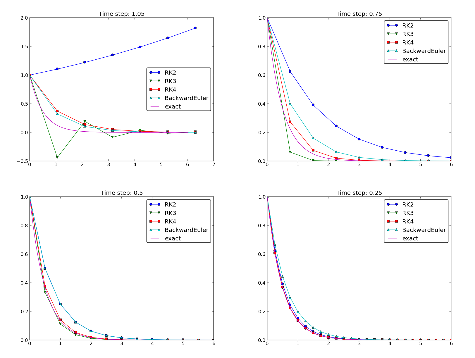
The 4-th order Runge-Kutta method (RK4) is the method of choice!
ode45).