
| Author: | Hans Petter Langtangen |
|---|---|
| Date: | Nov 29, 2013 |
This document presents a FEniCS tutorial to get new users quickly up and running with solving differential equations. FEniCS can be programmed both in C++ and Python, but this tutorial focuses exclusively on Python programming, since this is the simplest approach to exploring FEniCS for beginners and since it actually gives high performance. After having digested the examples in this tutorial, the reader should be able to learn more from the FEniCS documentation, the numerous demos, and the comprehensive FEniCS book Automated Solution of Differential Equations by the Finite element Method: The FEniCS book [Ref01].
The tutorial is still in an initial state so the reader is encouraged to send email to the author on hpl@simula.no about typos, errors, and suggestions for improvements.
Warning
This tutorial is compatible with FEniCS version 1.1. There are some differences between this document and the tutorial in the FEniCS book [Ref01] because of changes in the FEniCS software from version 1.0 to 1.1
FEniCS is a user-friendly tool for solving partial differential equations (PDEs). The goal of this tutorial is to get you started with FEniCS through a series of simple examples that demonstrate
- how to define the PDE problem in terms of a variational problem,
- how to define simple domains,
- how to deal with Dirichlet, Neumann, and Robin conditions,
- how to deal with variable coefficients,
- how to deal with domains built of several materials (subdomains),
- how to compute derived quantities like the flux vector field or a functional of the solution,
- how to quickly visualize the mesh, the solution, the flux, etc.,
- how to solve nonlinear PDEs in various ways,
- how to deal with time-dependent PDEs,
- how to set parameters governing solution methods for linear systems,
- how to create domains of more complex shape.
The mathematics of the illustrations is kept simple to better focus on FEniCS functionality and syntax. This means that we mostly use the Poisson equation and the time-dependent diffusion equation as model problems, often with input data adjusted such that we get a very simple solution that can be exactly reproduced by any standard finite element method over a uniform, structured mesh. This latter property greatly simplifies the verification of the implementations. Occasionally we insert a physically more relevant example to remind the reader that changing the PDE and boundary conditions to something more real might often be a trivial task.
FEniCS may seem to require a thorough understanding of the abstract mathematical version of the finite element method as well as familiarity with the Python programming language. Nevertheless, it turns out that many are able to pick up the fundamentals of finite elements and Python programming as they go along with this tutorial. Simply keep on reading and try out the examples. You will be amazed of how easy it is to solve PDEs with FEniCS!
Reading this tutorial obviously requires access to a machine where the FEniCS software is installed. The section Installing FEniCS explains briefly how to install the necessary tools.
All the examples discussed in the following are available as executable Python source code files in a directory tree.
Our first example regards the Poisson problem,
Here, \(u(\boldsymbol{x})\) is the unknown function, \(f(\boldsymbol{x})\) is a prescribed function, \(\nabla^2\) is the Laplace operator (also often written as \(\Delta\)), \(\Omega\) is the spatial domain, and \(\partial\Omega\) is the boundary of \(\Omega\). A stationary PDE like this, together with a complete set of boundary conditions, constitute a boundary-value problem, which must be precisely stated before it makes sense to start solving it with FEniCS.
In two space dimensions with coordinates \(x\) and \(y\), we can write out the Poisson equation as
The unknown \(u\) is now a function of two variables, \(u(x,y)\), defined over a two-dimensional domain \(\Omega\).
The Poisson equation arises in numerous physical contexts, including heat conduction, electrostatics, diffusion of substances, twisting of elastic rods, inviscid fluid flow, and water waves. Moreover, the equation appears in numerical splitting strategies of more complicated systems of PDEs, in particular the Navier-Stokes equations.
Solving a physical problem with FEniCS consists of the following steps:
- Identify the PDE and its boundary conditions.
- Reformulate the PDE problem as a variational problem.
- Make a Python program where the formulas in the variational problem are coded, along with definitions of input data such as \(f\), \(u_0\), and a mesh for the spatial domain \(\Omega\).
- Add statements in the program for solving the variational problem, computing derived quantities such as \(\nabla u\), and visualizing the results.
We shall now go through steps 2-4 in detail. The key feature of FEniCS is that steps 3 and 4 result in fairly short code, while most other software frameworks for PDEs require much more code and more technically difficult programming.
FEniCS makes it easy to solve PDEs if finite elements are used for discretization in space and the problem is expressed as a variational problem. Readers who are not familiar with variational problems will get a brief introduction to the topic in this tutorial, but getting and reading a proper book on the finite element method in addition is encouraged. The section Books on the Finite Element Method contains a list of some suitable books.
The core of the recipe for turning a PDE into a variational problem is to multiply the PDE by a function \(v\), integrate the resulting equation over \(\Omega\), and perform integration by parts of terms with second-order derivatives. The function \(v\) which multiplies the PDE is in the mathematical finite element literature called a test function. The unknown function \(u\) to be approximated is referred to as a trial function. The terms test and trial function are used in FEniCS programs too. Suitable function spaces must be specified for the test and trial functions. For standard PDEs arising in physics and mechanics such spaces are well known.
In the present case, we first multiply the Poisson equation by the test function \(v\) and integrate,
Then we apply integration by parts to the integrand with second-order derivatives,
where \({\partial u\over \partial n}\) is the derivative of \(u\) in the outward normal direction at the boundary. The test function \(v\) is required to vanish on the parts of the boundary where \(u\) is known, which in the present problem implies that \(v=0\) on the whole boundary \(\partial\Omega\). The second term on the right-hand side of the last equation therefore vanishes. It then follows that
This equation is supposed to hold for all \(v\) in some function space \(\hat V\). The trial function \(u\) lies in some (possibly different) function space \(V\). We say that the last equation is the weak form of the original boundary value problem consisting of the PDE \(-\nabla^2u=f\) and the boundary condition \(u=u_0\).
The proper statement of our variational problem now goes as follows: Find \(u \in V\) such that
The test and trial spaces \(\hat{V}\) and \(V\) are in the present problem defined as
In short, \(H^1(\Omega)\) is the mathematically well-known Sobolev space containing functions \(v\) such that \(v^2\) and \(||\nabla v||^2\) have finite integrals over \(\Omega\). The solution of the underlying PDE must lie in a function space where also the derivatives are continuous, but the Sobolev space \(H^1(\Omega)\) allows functions with discontinuous derivatives. This weaker continuity requirement of \(u\) in the variational statement, caused by the integration by parts, has great practical consequences when it comes to constructing finite elements.
To solve the Poisson equation numerically, we need to transform the continuous variational problem to a discrete variational problem. This is done by introducing finite-dimensional test and trial spaces, often denoted as \(\hat{V}_h\subset\hat{V}\) and \(V_h\subset{V}\). The discrete variational problem reads: Find \(u_h \in V_h \subset V\) such that
The choice of \(\hat{V}_h\) and \(V_h\) follows directly from the kind of finite elements we want to apply in our problem. For example, choosing the well-known linear triangular element with three nodes implies that \(\hat V_h\) and \(V_h\) are the spaces of all piecewise linear functions over a mesh of triangles, where the functions in \(\hat V_h\) are zero on the boundary and those in \(V_h\) equal \(u_0\) on the boundary.
The mathematics literature on variational problems writes \(u_h\) for the solution of the discrete problem and \(u\) for the solution of the continuous problem. To obtain (almost) a one-to-one relationship between the mathematical formulation of a problem and the corresponding FEniCS program, we shall use \(u\) for the solution of the discrete problem and \(u_{e}\) for the exact solution of the continuous problem, if we need to explicitly distinguish between the two. In most cases, we will introduce the PDE problem with \(u\) as unknown, derive a variational equation \(a(u,v)=L(v)\) with \(u\in V\) and \(v\in \hat V\), and then simply discretize the problem by saying that we choose finite-dimensional spaces for \(V\) and \(\hat V\). This restriction of \(V\) implies that \(u\) becomes a discrete finite element function. In practice, this means that we turn our PDE problem into a continuous variational problem, create a mesh and specify an element type, and then let \(V\) correspond to this mesh and element choice. Depending upon whether \(V\) is infinite- or finite-dimensional, \(u\) will be the exact or approximate solution.
It turns out to be convenient to introduce the following unified notation for linear weak forms:
In the present problem we have that
From the mathematics literature, \(a(u,v)\) is known as a bilinear form and \(L(v)\) as a linear form. We shall in every linear problem we solve identify the terms with the unknown \(u\) and collect them in \(a(u,v)\), and similarly collect all terms with only known functions in \(L(v)\). The formulas for \(a\) and \(L\) are then coded directly in the program.
To summarize, before making a FEniCS program for solving a PDE, we must first perform two steps:
- Turn the PDE problem into a discrete variational problem: find \(u\in V\) such that \(a(u,v) = L(v)\quad\forall v\in \hat{V}\).
- Specify the choice of spaces (\(V\) and \(\hat V\)), which means specifying the mesh and type of finite elements.
The test problem so far has a general domain \(\Omega\) and general functions \(u_0\) and \(f\). For our first implementation we must decide on specific choices of \(\Omega\), \(u_0\), and \(f\). It will be wise to construct a specific problem where we can easily check that the computed solution is correct. Let us start with specifying an exact solution
on some 2D domain. By inserting eq:ref:tut:poisson1:impl:uex in our Poisson problem, we find that \(u_{\rm e}(x,y)\) is a solution if
regardless of the shape of the domain. We choose here, for simplicity, the domain to be the unit square,
The reason for specifying the solution eq:ref:tut:poisson1:impl:uex is that the finite element method, with a rectangular domain uniformly partitioned into linear triangular elements, will exactly reproduce a second-order polynomial at the vertices of the cells, regardless of the size of the elements. This property allows us to verify the implementation by comparing the computed solution, called \(u\) in this document (except when setting up the PDE problem), with the exact solution, denoted by \(u_{\rm e}\): \(u\) should equal \(u_{\rm}\) to machine precision emph{at the nodes}. Test problems with this property will be frequently constructed throughout this tutorial.
A FEniCS program for solving the Poisson equation in 2D with the given choices of \(u_0\), \(f\), and \(\Omega\) may look as follows:
from dolfin import *

# Create mesh and define function space
mesh = UnitSquareMesh(6, 4)
#mesh = UnitCubeMesh(6, 4, 5)
V = FunctionSpace(mesh, 'Lagrange', 1)

# Define boundary conditions
u0 = Expression('1 + x[0]*x[0] + 2*x[1]*x[1]')

def u0_boundary(x, on_boundary):
    return on_boundary

bc = DirichletBC(V, u0, u0_boundary)

# Define variational problem
u = TrialFunction(V)
v = TestFunction(V)
f = Constant(-6.0)
a = inner(nabla_grad(u), nabla_grad(v))*dx
L = f*v*dx

# Compute solution
u = Function(V)
solve(a == L, u, bc)

# Plot solution and mesh
plot(u, interactive=True)
plot(mesh, interactive=True)

# Dump solution to file in VTK format
file = File('poisson.pvd')
file << u
The complete code can be found in the file d1_p2D.py in the directory stationary/poisson.
We shall now dissect this FEniCS program in detail. The program is written in the Python programming language. You may either take a quick look at the official Python tutorial to pick up the basics of Python if you are unfamiliar with the language, or you may learn enough Python as you go along with the examples in the present tutorial. The latter strategy has proven to work for many newcomers to FEniCS. (The requirement of using Python and an abstract mathematical formulation of the finite element problem may seem difficult for those who are unfamiliar with these topics. However, the amount of mathematics and Python that is really demanded to get you productive with FEniCS is quite limited. And Python is an easy-to-learn language that you certainly will love and use far beyond FEniCS programming.) the section Books on Python lists some relevant Python books.
The listed FEniCS program defines a finite element mesh, the discrete function spaces \(V\) and \(\hat{V}\) corresponding to this mesh and the element type, boundary conditions for \(u\) (the function \(u_0\)), \(a(u,v)\), and \(L(v)\). Thereafter, the unknown trial function \(u\) is computed. Then we can investigate \(u\) visually or analyze the computed values.
The first line in the program,
from dolfin import *
imports the key classes UnitSquareMesh, FunctionSpace, Function, and so forth, from the DOLFIN library. All FEniCS programs for solving PDEs by the finite element method normally start with this line. DOLFIN is a software library with efficient and convenient C++ classes for finite element computing, and dolfin is a Python package providing access to this C++ library from Python programs. You can think of FEniCS as an umbrella, or project name, for a set of computational components, where DOLFIN is one important component for writing finite element programs. The from dolfin import * statement imports other components too, but newcomers to FEniCS programming do not need to care about this.
The statement
mesh = UnitSquareMesh(6, 4)
defines a uniform finite element mesh over the unit square \([0,1]\times [0,1]\). The mesh consists of cells, which are triangles with straight sides. The parameters 6 and 4 tell that the square is first divided into \(6\times 4\) rectangles, and then each rectangle is divided into two triangles. The total number of triangles then becomes 48. The total number of vertices in this mesh is \(7\cdot 5=35\). DOLFIN offers some classes for creating meshes over very simple geometries. For domains of more complicated shape one needs to use a separate preprocessor program to create the mesh. The FEniCS program will then read the mesh from file.
Having a mesh, we can define a discrete function space V over this mesh:
V = FunctionSpace(mesh, 'Lagrange', 1)
The second argument reflects the type of element, while the third argument is the degree of the basis functions on the element.
The type of element is here “Lagrange”, implying the standard Lagrange family of elements. (Some FEniCS programs use 'CG', for Continuous Galerkin, as a synonym for 'Lagrange'.) With degree 1, we simply get the standard linear Lagrange element, which is a triangle with nodes at the three vertices. Some finite element practitioners refer to this element as the “linear triangle”. The computed \(u\) will be continuous and linearly varying in \(x\) and \(y\) over each cell in the mesh. Higher-degree polynomial approximations over each cell are trivially obtained by increasing the third parameter in FunctionSpace. Changing the second parameter to 'DG' creates a function space for discontinuous Galerkin methods.
In mathematics, we distinguish between the trial and test spaces \(V\) and \(\hat{V}\). The only difference in the present problem is the boundary conditions. In FEniCS we do not specify the boundary conditions as part of the function space, so it is sufficient to work with one common space V for the and trial and test functions in the program:
u = TrialFunction(V)
v = TestFunction(V)
The next step is to specify the boundary condition: \(u=u_0\) on \(\partial\Omega\). This is done by
bc = DirichletBC(V, u0, u0_boundary)
where u0 is an instance holding the \(u_0\) values, and u0_boundary is a function (or object) describing whether a point lies on the boundary where \(u\) is specified.
Boundary conditions of the type \(u=u_0\) are known as Dirichlet conditions, and also as essential boundary conditions in a finite element context. Naturally, the name of the DOLFIN class holding the information about Dirichlet boundary conditions is DirichletBC.
The u0 variable refers to an Expression object, which is used to represent a mathematical function. The typical construction is
u0 = Expression(formula)
where formula is a string containing the mathematical expression. This formula is written with C++ syntax (the expression is automatically turned into an efficient, compiled C++ function, see the section User-Defined Functions for details on the syntax). The independent variables in the function expression are supposed to be available as a point vector x, where the first element x[0] corresponds to the \(x\) coordinate, the second element x[1] to the \(y\) coordinate, and (in a three-dimensional problem) x[2] to the \(z\) coordinate. With our choice of \(u_0(x,y)=1 + x^2 + 2y^2\), the formula string must be written as 1 + x[0]*x[0] + 2*x[1]*x[1]:
u0 = Expression('1 + x[0]*x[0] + 2*x[1]*x[1]')
The information about where to apply the u0 function as boundary condition is coded in a function u0_boundary:
def u0_boundary(x, on_boundary):
    return on_boundary
A function like u0_boundary for marking the boundary must return a boolean value: True if the given point x lies on the Dirichlet boundary and False otherwise. The argument on_boundary is True if x is on the physical boundary of the mesh, so in the present case, where we are supposed to return True for all points on the boundary, we can just return the supplied value of on_boundary. The u0_boundary function will be called for every discrete point in the mesh, which allows us to have boundaries where \(u\) are known also inside the domain, if desired.
One can also omit the on_boundary argument, but in that case we need to test on the value of the coordinates in x:
def u0_boundary(x):
    return x[0] == 0 or x[1] == 0 or x[0] == 1 or x[1] == 1
As for the formula in Expression objects, x in the u0_boundary function represents a point in space with coordinates x[0], x[1], etc. Comparing floating-point values using an exact match test with == is not good programming practice, because small round-off errors in the computations of the x values could make a test x[0] == 1 become false even though x lies on the boundary. A better test is to check for equality with a tolerance:
def u0_boundary(x):
    tol = 1E-15
    return abs(x[0]) < tol or \
           abs(x[1]) < tol or \
           abs(x[0] - 1) < tol or \
           abs(x[1] - 1) < tol
Before defining \(a(u,v)\) and \(L(v)\) we have to specify the \(f\) function:
f = Expression('-6')
When \(f\) is constant over the domain, f can be more efficiently represented as a Constant object:
f = Constant(-6.0)
Now we have all the objects we need in order to specify this problem’s \(a(u,v)\) and \(L(v)\):
a = inner(nabla_grad(u), nabla_grad(v))*dx
L = f*v*dx
In essence, these two lines specify the PDE to be solved. Note the very close correspondence between the Python syntax and the mathematical formulas \(\nabla u\cdot\nabla v {\, \mathrm{d}x}\) and \(fv {\, \mathrm{d}x}\). This is a key strength of FEniCS: the formulas in the variational formulation translate directly to very similar Python code, a feature that makes it easy to specify PDE problems with lots of PDEs and complicated terms in the equations. The language used to express weak forms is called UFL (Unified Form Language) and is an integral part of FEniCS.
Instead of nabla_grad we could also just have written grad in the examples in this tutorial. However, when taking gradients of vector fields, grad and nabla_grad differ. The latter is consistent with the tensor algebra commonly used to derive vector and tensor PDEs, where \(\nabla\) (“nabla”) acts as a vector operator, and therefore this author prefers to always use nabla_grad.
Having a and L defined, and information about essential (Dirichlet) boundary conditions in bc, we can compute the solution, a finite element function u, by
u = Function(V)
solve(a == L, u, bc)
Some prefer to replace a and L by an equation variable, which is accomplished by this equivalent code:
equation = inner(nabla_grad(u), nabla_grad(v))*dx == f*v*dx
u = Function(V)
solve(equation, u, bc)
Note that we first defined the variable u as a TrialFunction and used it to represent the unknown in the form a. Thereafter, we redefined u to be a Function object representing the solution, i.e., the computed finite element function \(u\). This redefinition of the variable u is possible in Python and often done in FEniCS applications. The two types of objects that u refers to are equal from a mathematical point of view, and hence it is natural to use the same variable name for both objects. In a program, however, TrialFunction objects must always be used for the unknowns in the problem specification (the form a), while Function objects must be used for quantities that are computed (known).
The simplest way of quickly looking at u and the mesh is to say
plot(u)
plot(mesh)
interactive()
The interactive() call is necessary for the plot to remain on the screen. With the left, middle, and right mouse buttons you can rotate, translate, and zoom (respectively) the plotted surface to better examine what the solution looks like. Figures Plot of the solution in the first FEniCS example and Plot of the mesh in the first FEniCS example display the resulting \(u\) function and the finite element mesh, respectively.
It is also possible to dump the computed solution to file, e.g., in the VTK format:
file = File('poisson.pvd')
file << u
The poisson.pvd file can now be loaded into any front-end to VTK, say ParaView or VisIt. The plot function is intended for quick examination of the solution during program development. More in-depth visual investigations of finite element solutions will normally benefit from using highly professional tools such as ParaView and VisIt.
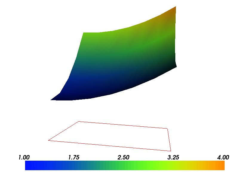
Plot of the solution in the first FEniCS example
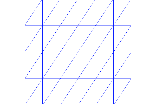
Plot of the mesh in the first FEniCS example
The next three sections deal with some technicalities about specifying the solution method for linear systems (so that you can solve large problems) and examining array data from the computed solution (so that you can check that the program is correct). These technicalities are scattered around in forthcoming programs. However, the impatient reader who is more interested in seeing the previous program being adapted to a real physical problem, and play around with some interesting visualizations, can safely jump to the section Solving a Real Physical Problem. Information in the intermediate sections can be studied on demand.
Sparse LU decomposition (Gaussian elimination) is used by default to solve linear systems of equations in FEniCS programs. This is a very robust and recommended method for a few thousand unknowns in the equation system, and may hence be the method of choice in many 2D and smaller 3D problems. However, sparse LU decomposition becomes slow and memory demanding in large problems. This fact forces the use of iterative methods, which are faster and require much less memory.
Preconditioned Krylov solvers is a type of popular iterative methods that are easily accessible in FEniCS programs. The Poisson equation results in a symmetric, positive definite coefficient matrix, for which the optimal Krylov solver is the Conjugate Gradient (CG) method. Incomplete LU factorization (ILU) is a popular and robust all-round preconditioner, so let us try the CG-ILU pair:
solve(a == L, u, bc)
      solver_parameters={'linear_solver': 'cg',
                         'preconditioner': 'ilu'})
# Alternative syntax
solve(a == L, u, bc,
      solver_parameters=dict(linear_solver='cg',
                             preconditioner='ilu'))
the section Linear Solvers and Preconditioners lists the most popular choices of Krylov solvers and preconditioners available in FEniCS
The actual CG and ILU implementations that are brought into action depends on the choice of linear algebra package. FEniCS interfaces several linear algebra packages, called linear algebra backends in FEniCS terminology. PETSc is the default choice if DOLFIN is compiled with PETSc, otherwise uBLAS. Epetra (Trilinos) and MTL4 are two other supported backends. Which backend to apply can be controlled by setting
parameters['linear_algebra_backend'] = backendname
where backendname is a string, either 'PETSc', 'uBLAS', 'Epetra', or 'MTL4'. All these backends offer high-quality implementations of both iterative and direct solvers for linear systems of equations.
A common platform for FEniCS users is Ubuntu Linux. The FEniCS distribution for Ubuntu contains PETSc, making this package the default linear algebra backend. The default solver is sparse LU decomposition ('lu'), and the actual software that is called is then the sparse LU solver from UMFPACK (which PETSc has an interface to). The MTL4 package is not available in Ubuntu, so this choice of backend unavailable to FEniCS users on Ubuntu unless they build FEniCS from the source code. There is a tool Dorsal that performs the build process automatically. The available linear algebra backends in a FEniCS installation is listed by
list_linear_algebra_backends()
We will normally like to control the tolerance in the stopping criterion and the maximum number of iterations when running an iterative method. Such parameters can be set by accessing the global parameter database, which is called parameters and which behaves as a nested dictionary. Write
info(parameters, True)
to list all parameters and their default values in the database. The nesting of parameter sets is indicated through indentation in the output from info. According to this output, the relevant parameter set is named 'krylov_solver', and the parameters are set like this:
prm = parameters['krylov_solver'] # short form
prm['absolute_tolerance'] = 1E-10
prm['relative_tolerance'] = 1E-6
prm['maximum_iterations'] = 1000
Stopping criteria for Krylov solvers usually involve the norm of the residual, which must be smaller than the absolute tolerance parameter or smaller than the relative tolerance parameter times the initial residual.
To see the number of actual iterations to reach the stopping criterion, we can insert
set_log_level(PROGRESS)
# or
set_log_level(DEBUG)
A message with the equation system size, solver type, and number of iterations arises from specifying the argument PROGRESS, while DEBUG results in more information, including CPU time spent in the various parts of the matrix assembly and solve process.
The complete solution process with control of the solver parameters now contains the statements
prm = parameters['krylov_solver'] # short form
prm['absolute_tolerance'] = 1E-10
prm['relative_tolerance'] = 1E-6
prm['maximum_iterations'] = 1000
set_log_level(PROGRESS)

solve(a == L, u, bc,
      solver_parameters={'linear_solver': 'cg',
                         'preconditioner': 'ilu'})
The demo program d2_p2D.py in the stationary/poisson directory incorporates the above shown control of the linear solver and precnditioner, but is otherwise similar to the previous d1_p2D.py program.
We remark that default values for the global parameter database can be defined in an XML file, see the example file dolfin_parameters.xml in the directory stationary/poisson. If such a file is found in the directory where a FEniCS program is run, this file is read and used to initialize the parameters object. Otherwise, the file .config/fenics/dolfin_parameters.xml in the user’s home directory is read, if it exists. The XML file can also be in gzip’ed form with the extension .xml.gz.
The solve(a == L, u, bc) call is just a compact syntax alternative to a slightly more comprehensive specification of the variational equation and the solution of the associated linear system. This alternative syntax is used in a lot of FEniCS applications and will also be used later in this tutorial, so we show it already now:
u = Function(V)
problem = LinearVariationalProblem(a, L, u, bc)
solver  = LinearVariationalSolver(problem)
solver.solve()
Many objects have an attribute parameters corresponding to a parameter set in the global parameters database, but local to the object. Here, solver.parameters play that role. Setting the CG method with ILU preconditiong as solution method and specifying solver-specific parameters can be done like this:
solver.parameters['linear_solver'] = 'cg'
solver.parameters['preconditioner'] = 'ilu'
cg_prm = solver.parameters['krylov_solver'] # short form
cg_prm['absolute_tolerance'] = 1E-7
cg_prm['relative_tolerance'] = 1E-4
cg_prm['maximum_iterations'] = 1000
Calling info(solver.parameters, True) lists all the available parameter sets with default values for each parameter. Settings in the global parameters database are propagated to parameter sets in individual objects, with the possibility of being overwritten as done above.
The d3_p2D.py program modifies the d2_p2D.py file to incorporate objects for the variational problem and solver.
We know that, in the particular boundary-value problem of the section Implementation (1), the computed solution \(u\) should equal the exact solution at the vertices of the cells. An important extension of our first program is therefore to examine the computed values of the solution, which is the focus of the present section.
A finite element function like \(u\) is expressed as a linear combination of basis functions \(\phi_j\), spanning the space \(V\):
By writing solve(a == L, u, bc) in the program, a linear system will be formed from \(a\) and \(L\), and this system is solved for the \(U_1,\ldots,U_N\) values. The \(U_1,\ldots,U_N\) values are known
as degrees of freedom of \(u\). For Lagrange elements (and many other element types) \(U_k\) is simply the value of \(u\) at the node with global number \(k\). (The nodes and cell vertices coincide for linear Lagrange elements, while for higher-order elements there may be additional nodes at the facets and in the interior of cells.)
Having u represented as a Function object, we can either evaluate u(x) at any vertex x in the mesh, or we can grab all the values \(U_j\) directly by
u_nodal_values = u.vector()
The result is a DOLFIN Vector object, which is basically an encapsulation of the vector object used in the linear algebra package that is used to solve the linear system arising from the variational problem. Since we program in Python it is convenient to convert the Vector object to a standard numpy array for further processing:
u_array = u_nodal_values.array()
With numpy arrays we can write “MATLAB-like” code to analyze the data. Indexing is done with square brackets: u_array[i], where the index i always starts at 0.
Mesh information can be gathered from the mesh object, e.g.,
- mesh.coordinates() returns the coordinates of the vertices as a numpy array with shape (number of vertices, number of space dimensions), \(M\) being the number of vertices in the mesh and \(d\) being the number of space dimensions,
- mesh.num_cells() returns the number of cells (triangles) in the mesh,
- mesh.num_vertices() returns the number of vertices in the mesh (with our choice of linear Lagrange elements this equals the number of nodes),
- mesh.cells() returns the vertex numbers of the vertices in each cell as a numpy array with shape (number of cells, number of vertices in a cell),
- mesh.hmin() returns the minimum cell diameter (“smallest cell”),
- mesh.hmax() returns the maximum cell diameter (“largest cell”).
Writing print mesh dumps a short, “pretty print” description of the mesh (print mesh actually displays the result of str(mesh)`, which defines the pretty print):
<Mesh of topological dimension 2 (triangles) with
16 vertices and 18 cells, ordered>
All mesh objects are of type Mesh so typing the command pydoc dolfin.Mesh in a terminal window will give a list of methods (that is, functions in a class) that can be called through any Mesh object. In fact, pydoc dolfin.X shows the documentation of any DOLFIN name X.
Writing out the solution on the screen can now be done by a simple loop:
coor = mesh.coordinates()
if mesh.num_vertices() == len(u_array):
    for i in range(mesh.num_vertices()):
        print 'u(%8g,%8g) = %g' % (coor[i][0], coor[i][1], u_array[i])
The beginning of the output looks like this:
u(       0,       0) = 1
u(0.166667,       0) = 1.02778
u(0.333333,       0) = 1.11111
u(     0.5,       0) = 1.25
u(0.666667,       0) = 1.44444
u(0.833333,       0) = 1.69444
u(       1,       0) = 2
For Lagrange elements of degree higher than one, the vertices do not correspond to all the nodal points and the if-test fails.
For verification purposes we want to compare the values of the computed u at the nodes (given by u_array) with the exact solution u0 evaluated at the nodes. The difference between the computed and exact solution should be less than a small tolerance at all the nodes. The Expression object u0 can be evaluated at any point x by calling u0(x). Specifically, u0(coor[i]) returns the value of u0 at the vertex or node with global number i.
Alternatively, we can make a finite element field u_e, representing the exact solution, whose values at the nodes are given by the u0 function. With mathematics, \(u_{\mbox{e}} = \sum_{j=1}^N E_j\phi_j\), where \(E_j=u_0(x_j,y_j)\), \((x_j,y_j)\) being the coordinates of node number \(j\). This process is known as interpolation. FEniCS has a function for performing the operation:
u_e = interpolate(u0, V)
The maximum error can now be computed as
u_e_array = u_e.vector().array()
print 'Max error:', numpy.abs(u_e_array - u_array).max()
The value of the error should be at the level of the machine precision (\(10^{-16}\)).
To demonstrate the use of point evaluations of Function objects, we write out the computed u at the center point of the domain and compare it with the exact solution:
center = (0.5, 0.5)
print 'numerical u at the center point:',  u(center)
print 'exact     u at the center point:', u0(center)
Trying a \(3\times 3\) mesh, the output from the previous snippet becomes
numerical u at the center point: [ 1.83333333]
exact     u at the center point: [ 1.75]
The discrepancy is due to the fact that the center point is not a node in this particular mesh, but a point in the interior of a cell, and u varies linearly over the cell while u0 is a quadratic function.
We have seen how to extract the nodal values in a numpy array. If desired, we can adjust the nodal values too. Say we want to normalize the solution such that \(\max_j U_j = 1\). Then we must divide all \(U_j\) values by \(\max_j U_j\). The following snippet performs the task:
max_u = u_array.max()
u_array /= max_u
u.vector()[:] = u_array
u.vector().set_local(u_array)  # alternative
print u.vector().array()
That is, we manipulate u_array as desired, and then we insert this array into u‘s Vector object. The /= operator implies an in-place modification of the object on the left-hand side: all elements of the u_array are divided by the value max_u. Alternatively, one could write u_array = u_array/max_u, which implies creating a new array on the right-hand side and assigning this array to the name u_array.
A call like u.vector().array() returns a copy of the data in u.vector(). One must therefore never perform assignments like u.vector.array()[:] = ..., but instead extract the numpy array (i.e., a copy), manipulate it, and insert it back with u.vector()[:] = `` or ``u.set_local(...).
All the code in this subsection can be found in the file d4_p2D.py in the stationary/poisson directory. We have commented out the plotting statements in this version of the program, but if you want plotting to happen, make sure that interactive is called at the very end of the program.
Perhaps you are not particularly amazed by viewing the simple surface of \(u\) in the test problem from the section Implementation (1). However, solving a real physical problem with a more interesting and amazing solution on the screen is only a matter of specifying a more exciting domain, boundary condition, and/or right-hand side \(f\).
One possible physical problem regards the deflection \(D(x,y)\) of an elastic circular membrane with radius \(R\), subject to a localized perpendicular pressure force, modeled as a Gaussian function. The appropriate PDE model is
with
Here, \(T\) is the tension in the membrane (constant), \(p\) is the external pressure load, \(A\) the amplitude of the pressure, \((x_0,y_0)\) the localization of the Gaussian pressure function, and \(\sigma\) the “width” of this function. The boundary of the membrane has no deflection, implying \(D=0\) as boundary condition.
For scaling and verification it is convenient to simplify the problem to find an analytical solution. In the limit \(\sigma\rightarrow\infty\), \(p\rightarrow A/(2\pi\sigma)\), which allows us to integrate an axi-symmetric version of the equation in the radial coordinate \(r\in [0,R]\) and obtain \(D(r)=(r^2-R^2)A/(8\pi\sigma T)\). This result gives a rough estimate of the characteristic size of the deflection: \(|D(0)|=AR^2/(8\pi\sigma T)\), which can be used to scale the deflecton. With \(R\) as characteristic length scale, we can derive the equivalent dimensionless problem on the unit circle,
with \(w=0\) on the boundary and with
For notational convenience we have dropped introducing new symbols for the scaled coordinates in (13). Now \(D\) is related to \(w\) through \(D = AR^2w/(8\pi\sigma T)\).
Let us list the modifications of the d1_p2D.py program that are needed to solve this membrane problem:
- Initialize \(T\), \(A\), \(R\), \(x_0\), \(y_0\), and \(\sigma\),
- create a mesh over the unit circle,
- make an expression object for the scaled pressure function \(f\),
- define the a and L formulas in the variational problem for \(w\) and compute the solution,
- plot the mesh, \(w\), and \(f\),
- write out the maximum real deflection \(D\).
Some suitable values of \(T\), \(A\), \(R\), \(x_0\), \(y_0\), and \(\sigma\) are
T = 10.0  # tension
A = 1.0   # pressure amplitude
R = 0.3   # radius of domain
theta = 0.2
x0 = 0.6*R*cos(theta)
y0 = 0.6*R*sin(theta)
sigma = 0.025
A mesh over the unit circle can be created by
mesh = UnitCircleMesh(n)
where n is the typical number of elements in the radial direction.
The function \(f\) is represented by an Expression object. There are many physical parameters in the formula for \(f\) that enter the expression string and these parameters must have their values set by keyword arguments:
f = Expression('4*exp(-0.5*(pow((R*x[0] - x0)/sigma, 2)) '
               '     - 0.5*(pow((R*x[1] - y0)/sigma, 2)))',
               R=R, x0=x0, y0=y0, sigma=sigma)
The coordinates in Expression objects must be a vector with indices 0, 1, and 2, and with the name x. Otherwise we are free to introduce names of parameters as long as these are given default values by keyword arguments. All the parameters initialized by keyword arguments can at any time have their values modified. For example, we may set
f.sigma = 50
f.x0 = 0.3
It would be of interest to visualize \(f\) along with \(w\) so that we can examine the pressure force and its response. We must then transform the formula (Expression) to a finite element function (Function). The most natural approach is to construct a finite element function whose degrees of freedom (values at the nodes in this case) are calculated from \(f\). That is, we interpolate \(f\) (see the section Examining the Discrete Solution):
f = interpolate(f, V)
Calling plot(f) will produce a plot of \(f\). Note that the assignment to f destroys the previous Expression object f, so if it is of interest to still have access to this object, another name must be used for the Function object returned by interpolate.
We need some evidence that the program works, and to this end we may use the analytical solution listed above for the case \(\sigma\rightarrow\infty\). In scaled coordinates the solution reads
Practical values for an infinite \(\sigma\) may be 50 or larger, and in such cases the program will report the maximum deviation between the computed \(w\) and the (approximate) exact \(w_{\rm e}\).
Note that the variational formulation remains the same as in the program from the section Implementation (1), except that \(u\) is replaced by \(w\) and \(u_0=0\). The final program is found in the file membrane1.py, located in the stationary/poisson directory, and also listed below. We have inserted capabilities for iterative solution methods and hence large meshes (the section Controlling the Solution Process), used objects for the variational problem and solver (the section Linear Variational Problem and Solver Objects), and made numerical comparison of the numerical and (approximate) analytical solution (the section Examining the Discrete Solution).
from dolfin import *
import numpy

# Set pressure function:
T = 10.0  # tension
A = 1.0   # pressure amplitude
R = 0.3   # radius of domain
theta = 0.2
x0 = 0.6*R*cos(theta)
y0 = 0.6*R*sin(theta)
sigma = 0.025
sigma = 50  # large value for verification
n = 40   # approx no of elements in radial direction
mesh = UnitCircleMesh(n)
V = FunctionSpace(mesh, 'Lagrange', 1)

# Define boundary condition w=0
def boundary(x, on_boundary):
    return on_boundary

bc = DirichletBC(V, Constant(0.0), boundary)

# Define variational problem
w = TrialFunction(V)
v = TestFunction(V)
a = inner(nabla_grad(w), nabla_grad(v))*dx
f = Expression('4*exp(-0.5*(pow((R*x[0] - x0)/sigma, 2)) '
               '      -0.5*(pow((R*x[1] - y0)/sigma, 2)))',
               R=R, x0=x0, y0=y0, sigma=sigma)
L = f*v*dx

# Compute solution
w = Function(V)
problem = LinearVariationalProblem(a, L, w, bc)
solver  = LinearVariationalSolver(problem)
solver.parameters['linear_solver'] = 'cg'
solver.parameters['preconditioner'] = 'ilu'
solver.solve()

# Plot scaled solution, mesh and pressure
plot(mesh, title='Mesh over scaled domain')
plot(w, title='Scaled deflection')
f = interpolate(f, V)
plot(f, title='Scaled pressure')

# Find maximum real deflection
max_w = w.vector().array().max()
max_D = A*max_w/(8*pi*sigma*T)
print 'Maximum real deflection is', max_D

# Verification for "flat" pressure (large sigma)
if sigma >= 50:
    w_e = Expression("1 - x[0]*x[0] - x[1]*x[1]")
    w_e = interpolate(w_e, V)
    dev = numpy.abs(w_e.vector().array() - w.vector().array()).max()
    print 'sigma=%g: max deviation=%e' % (sigma, dev)

# Should be at the end
interactive()
Choosing a small width \(\sigma\) (say 0.01) and a location \((x_0,y_0)\) toward the circular boundary (say \((0.6R\cos\theta, 0.6R\sin\theta)\) for any \(\theta\in [0,2\pi]\)), may produce an exciting visual comparison of \(w\) and \(f\) that demonstrates the very smoothed elastic response to a peak force (or mathematically, the smoothing properties of the inverse of the Laplace operator). One needs to experiment with the mesh resolution to get a smooth visual representation of~$f$. You are strongly encouraged to play around with the plots and different mesh resolutions.
As we go along with examples it is fun to play around with plot commands and visualize what is computed. This section explains some useful visualization features.
The plot command applies the VTK package to visualize finite element functions in a very quick and simple way. The command is ideal for debugging, teaching, and initial scientific investigations. The visualization can be interactive, or you can steer and automate it through program statements. More advanced and professional visualizations are usually better created with advanced tools like Mayavi, ParaView, or VisIt.
We have made a program membrane1v.py for the membrane deflection problem in the section Solving a Real Physical Problem and added various demonstrations of plotting capabilities. You are encouraged to play around with membrane1v.py and modify the code as you read about various features.
The plot function can take additional arguments, such as a title of the plot, or a specification of a wireframe plot (elevated mesh) instead of a colored surface plot:
plot(mesh, title='Finite element mesh')
plot(w, wireframe=True, title='solution')
The left mouse button is used to rotate the surface, while the right button can zoom the image in and out. Point the mouse to the Help text down in the lower left corner to get a list of all the keyboard commands that are available. For example,
- pressing m turns visualization of the mesh on and off,
- pressing b turns on and off a bounding box,
- pressing p dumps the plot to a PNG file,
- pressing P dumps the plot to a PDF file,
- pressing Ctrl +’ stretches the surface in the :math:`z direction,
- pressing Ctrl -‘ shrinks++ the surface in the :math:`z direction,
- pressing `Ctrl w’ closes the plot window,
- pressing `Ctrl q’ closes all plot windows.
The plots created by pressing p or P are stored in files with names dolfin_plot_X.png or dolfin_plot_X.pdf, where X is an integer that is increase by one from the last plot that was made. The file stem dolfin_plot_ can be set to something more suitable through the prefix keyword argument to plot, for instance, plot(f, prefix='pressure').
The plot function takes several other keyword arguments:
viz_w = plot(w,
             mode='warp',     # 'color' gives flat color plot
             wireframe=False, # True: elevated mesh
             title='Scaled membrane deflection',
             scale=3.0,       # stretch z axis by a factor of 3
             elevate=-75.0,   # tilt camera -75 degrees
             scalarbar=True,  # show colorbar
             axes=False,      # do not show X, Y, Z axes
             window_width=800,
             window_height=600,
             )
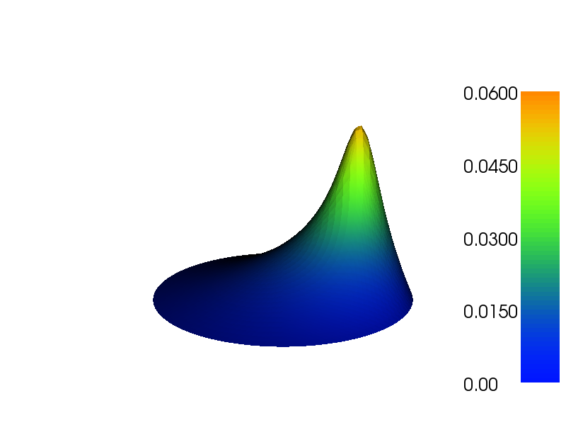
Figure Plot of the deflection of a membrane shows the resulting scalar surface.
By grabbing the plotting object created by the plot function we can create a PNG and PDF plot in the program:
viz_w.write_png('membrane_deflection')
viz_w.write_pdf('tmp')
# Rotate pdf file (right) from landscape to portrait
import os
os.system('pdftk tmp.pdf cat 1-endR output membrane_deflection.pdf')
Plot of the deflection of a membrane
In Poisson and many other problems the gradient of the solution is of interest. The computation is in principle simple: since \(u = \sum_{j=1}^N U_j \phi_j\), we have that
Given the solution variable u in the program, its gradient is obtained by grad(u) or nabla_grad(u). However, the gradient of a piecewise continuous finite element scalar field is a discontinuous vector field since the \(\phi_j\) has discontinuous derivatives at the boundaries of the cells. For example, using Lagrange elements of degree 1, \(u\) is linear over each cell, and the numerical \(\nabla u\) becomes a piecewise constant vector field. On the contrary, the exact gradient is continuous. For visualization and data analysis purposes we often want the computed gradient to be a continuous vector field. Typically, we want each component of \(\nabla u\) to be represented in the same way as \(u\) itself. To this end, we can project the components of \(\nabla u\) onto the same function space as we used for \(u\). This means that we solve \(w = \nabla u\) approximately by a finite element method, using the same elements for the components of \(w\) as we used for \(u\). This process is known as projection.
Looking at the component \(\partial u/\partial x\) of the gradient, we project the (discrete) derivative \(\sum_jU_j{\partial \phi_j/\partial x}\) onto a function space with basis \(\phi_1,\phi_2,\ldots\) such that the derivative in this space is expressed by the standard sum \(\sum_j\bar U_j \phi_j\), for suitable (new) coefficients \(\bar U_j\).
The variational problem for \(w\) reads: find \(w\in V^{(\mbox{g})}\) such that
where
The function spaces \(V^{(\mbox{g})}\) and \(\hat{V^{(\mbox{g})}}\) (with the superscript g denoting “gradient”) are vector versions of the function space for \(u\), with boundary conditions removed (if \(V\) is the space we used for \(u\), with no restrictions on boundary values, \(V^{(\mbox{g})} = \hat{V^{(\mbox{g})}} = [V]^d\), where \(d\) is the number of space dimensions). For example, if we used piecewise linear functions on the mesh to approximate \(u\), the variational problem for \(w\) corresponds to approximating each component field of \(w\) by piecewise linear functions.
The variational problem for the vector field \(w\), called grad_u in the code, is easy to solve in FEniCS:
V_g = VectorFunctionSpace(mesh, 'Lagrange', 1)
w = TrialFunction(V_g)
v = TestFunction(V_g)

a = inner(w, v)*dx
L = inner(grad(u), v)*dx
grad_u = Function(V_g)
solve(a == L, grad_u)

plot(grad_u, title='grad(u)')
The boundary condition argument to solve is dropped since there are no essential boundary conditions in this problem. The new thing is basically that we work with a VectorFunctionSpace, since the unknown is now a vector field, instead of the FunctionSpace object for scalar fields. Figure Example of visualizing the vector field :math:`nabla u` by arrows at the nodes shows example of how such a vector field is visualized.
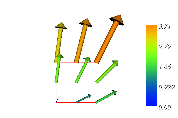
Example of visualizing the vector field :math:`nabla u` by arrows at the nodes
The scalar component fields of the gradient can be extracted as separate fields and, e.g., visualized:
grad_u_x, grad_u_y = grad_u.split(deepcopy=True)  # extract components
plot(grad_u_x, title='x-component of grad(u)')
plot(grad_u_y, title='y-component of grad(u)')
The deepcopy=True argument signifies a deep copy, which is a general term in computer science implying that a copy of the data is returned. (The opposite, deepcopy=False, means a shallow copy, where the returned objects are just pointers to the original data.)
The grad_u_x and grad_u_y variables behave as Function objects. In particular, we can extract the underlying arrays of nodal values by
grad_u_x_array = grad_u_x.vector().array()
grad_u_y_array = grad_u_y.vector().array()
The degrees of freedom of the grad_u vector field can also be reached by
grad_u_array = grad_u.vector().array()
but this is a flat numpy array where the degrees of freedom for the \(x\) component of the gradient is stored in the first part, then the degrees of freedom of the \(y\) component, and so on.
The program d5_p2D.py extends the code d5_p2D.py from the section Examining the Discrete Solution with computations and visualizations of the gradient. Examining the arrays grad_u_x_array and grad_u_y_array, or looking at the plots of grad_u_x and grad_u_y, quickly reveals that the computed grad_u field does not equal the exact gradient \((2x, 4y)\) in this particular test problem where \(u=1+x^2+2y^2\). There are inaccuracies at the boundaries, arising from the approximation problem for \(w\). Increasing the mesh resolution shows, however, that the components of the gradient vary linearly as \(2x\) and \(4y\) in the interior of the mesh (i.e., as soon as we are one element away from the boundary). See the section Quick Visualization with VTK for illustrations of this phenomenon.
Projecting some function onto some space is a very common operation in finite element programs. The manual steps in this process have therefore been collected in a utility function project(q, W), which returns the projection of some Function or Expression object named q onto the FunctionSpace or VectorFunctionSpace named W. Specifically, the previous code for projecting each component of grad(u) onto the same space that we use for u, can now be done by a one-line call
grad_u = project(grad(u), VectorFunctionSpace(mesh, 'Lagrange', 1))
The applications of projection are many, including turning discontinuous gradient fields into continuous ones, comparing higher- and lower-order function approximations, and transforming a higher-order finite element solution down to a piecewise linear field, which is required by many visualization packages.
Suppose we have a variable coefficient \(p(x,y)\) in the Laplace operator, as in the boundary-value problem
We shall quickly demonstrate that this simple extension of our model problem only requires an equally simple extension of the FEniCS program.
Let us continue to use our favorite solution \(u(x,y)=1+x^2+2y^2\) and then prescribe \(p(x,y)=x+y\). It follows that \(u_0(x,y) = 1 + x^2 + 2y^2\) and \(f(x,y)=-8x-10y\).
What are the modifications we need to do in the d4_p2D.py program from the section Examining the Discrete Solution?
- f must be an Expression since it is no longer a constant,
- a new Expression p must be defined for the variable coefficient,
- the variational problem is slightly changed.
First we address the modified variational problem. Multiplying the PDE by a test function \(v\) and integrating by parts now results in
The function spaces for \(u\) and \(v\) are the same as in the section Variational Formulation, implying that the boundary integral vanishes since \(v=0\) on \(\partial\Omega\) where we have Dirichlet conditions. The weak form \(a(u,v)=L(v)\) then has
In the code from the section Implementation (1) we must replace
a = inner(nabla_grad(u), nabla_grad(v))*dx
by
a = p*inner(nabla_grad(u), nabla_grad(v))*dx
The definitions of p and f read
p = Expression('x[0] + x[1]')
f = Expression('-8*x[0] - 10*x[1]')
No additional modifications are necessary. The complete code can be found in in the file vcp2D.py (variable-coefficient Poisson problem in 2D). You can run it and confirm that it recovers the exact \(u\) at the nodes.
The flux \(-p\nabla u\) may be of particular interest in variable-coefficient Poisson problems as it often has an interesting physical significance. As explained in the section Computing Derivatives, we normally want the piecewise discontinuous flux or gradient to be approximated by a continuous vector field, using the same elements as used for the numerical solution \(u\). The approximation now consists of solving \(w = -p\nabla u\) by a finite element method: find \(w\in V^{(\mbox{g})}\) such that
where
This problem is identical to the one in the section Computing Derivatives, except that \(p\) enters the integral in \(L\).
The relevant Python statements for computing the flux field take the form
V_g = VectorFunctionSpace(mesh, 'Lagrange', 1)
w = TrialFunction(V_g)
v = TestFunction(V_g)

a = inner(w, v)*dx
L = inner(-p*grad(u), v)*dx
flux = Function(V_g)
solve(a == L, flux)
The following call to project is equivalent to the above statements:
flux = project(-p*grad(u),
               VectorFunctionSpace(mesh, 'Lagrange', 1))
Plotting the flux vector field is naturally as easy as plotting the gradient (see the section Computing Derivatives):
plot(flux, title='flux field')

flux_x, flux_y = flux.split(deepcopy=True)  # extract components
plot(flux_x, title='x-component of flux (-p*grad(u))')
plot(flux_y, title='y-component of flux (-p*grad(u))')
For data analysis of the nodal values of the flux field we can grab the underlying numpy arrays:
flux_x_array = flux_x.vector().array()
flux_y_array = flux_y.vector().array()
The program vcp2D.py contains in addition some plots, including a curve plot comparing flux_x and the exact counterpart along the line \(y=1/2\). The associated programming details related to this visualization are explained in the section Visualization of Structured Mesh Data.
After the solution \(u\) of a PDE is computed, we occasionally want to compute functionals of \(u\), for example,
which often reflects some energy quantity. Another frequently occurring functional is the error
where \(u_{\rm e}\) is the exact solution. The error is of particular interest when studying convergence properties. Sometimes the interest concerns the flux out of a part \(\Gamma\) of the boundary \(\partial\Omega\),
where \(\boldsymbol{n}\) is an outward unit normal at \(\Gamma\) and \(p\) is a coefficient (see the problem in the section A Variable-Coefficient Poisson Problem for a specific example). All these functionals are easy to compute with FEniCS, and this section describes how it can be done.
Energy Functional. The integrand of the energy functional \({1\over2}\int_\Omega \nabla u\cdot \nabla u {\, \mathrm{d}x}\) is described in the UFL language in the same manner as we describe weak forms:
energy = 0.5*inner(grad(u), grad(u))*dx
E = assemble(energy)
The assemble call performs the integration. It is possible to restrict the integration to subdomains, or parts of the boundary, by using a mesh function to mark the subdomains as explained in the section Multiple Neumann, Robin, and Dirichlet Condition. The program membrane2.py carries out the computation of the elastic energy
in the membrane problem from the section Solving a Real Physical Problem.
Convergence Estimation. To illustrate error computations and convergence of finite element solutions, we modify the d5_p2D.py program from the section Computing Derivatives and specify a more complicated solution,
on the unit square. This choice implies \(f(x,y)=2\omega^2\pi^2 u(x,y)\). With \(\omega\) restricted to an integer it follows that \(u_0=0\).
We need to define the appropriate boundary conditions, the exact solution, and the \(f\) function in the code:
def boundary(x, on_boundary):
    return on_boundary

bc = DirichletBC(V, Constant(0.0), boundary)

omega = 1.0
u_e = Expression('sin(omega*pi*x[0])*sin(omega*pi*x[1])',
                 omega=omega)

f = 2*pi**2*omega**2*u_e
The computation of \(\left(\int_\Omega (u_e-u)^2 {\, \mathrm{d}x}\right)^{1/2}\) can be done by
error = (u - u_e)**2*dx
E = sqrt(assemble(error))
Here, u_e will be interpolated onto the function space V. This implies that the exact solution used in the integral will vary linearly over the cells, and not as a sine function, if V corresponds to linear Lagrange elements. This situation may yield a smaller error u - u_e than what is actually true.
More accurate representation of the exact solution is easily achieved by interpolating the formula onto a space defined by higher-order elements, say of third degree:
Ve = FunctionSpace(mesh, 'Lagrange', degree=3)
u_e_Ve = interpolate(u_e, Ve)
error = (u - u_e_Ve)**2*dx
E = sqrt(assemble(error))
To achieve complete mathematical control of which function space the computations are carried out in, we can explicitly interpolate u to the same space:
u_Ve = interpolate(u, Ve)
error = (u_Ve - u_e_Ve)**2*dx
The square in the expression for error will be expanded and lead to a lot of terms that almost cancel when the error is small, with the potential of introducing significant round-off errors. The function errornorm is available for avoiding this effect by first interpolating u and u_e to a space with higher-order elements, then subtracting the degrees of freedom, and then performing the integration of the error field. The usage is simple:
E = errornorm(u_e, u, normtype='L2', degree=3)
It is illustrative to look at the short implementation of errornorm:
def errornorm(u_e, u, Ve):
    u_Ve = interpolate(u, Ve)
    u_e_Ve = interpolate(u_e, Ve)
    e_Ve = Function(Ve)
    # Subtract degrees of freedom for the error field
    e_Ve.vector()[:] = u_e_Ve.vector().array() - \
                       u_Ve.vector().array()
    error = e_Ve**2*dx
    return sqrt(assemble(error))
The errornorm procedure turns out to be identical to computing the expression (u_e - u)**2*dx directly in the present test case.
Sometimes it is of interest to compute the error of the gradient field: \(||\nabla (u-u_{\mbox{e}})||\) (often referred to as the \(H^1\) seminorm of the error). Given the error field e_Ve above, we simply write
H1seminorm = sqrt(assemble(inner(grad(e_Ve), grad(e_Ve))*dx))
Finally, we remove all plot calls and printouts of \(u\) values in the original program, and collect the computations in a function:
def compute(nx, ny, degree):
    mesh = UnitSquareMesh(nx, ny)
    V = FunctionSpace(mesh, 'Lagrange', degree=degree)
    ...
    Ve = FunctionSpace(mesh, 'Lagrange', degree=5)
    E = errornorm(u_e, u, Ve)
    return E
Calling compute for finer and finer meshes enables us to study the convergence rate. Define the element size \(h=1/n\), where \(n\) is the number of divisions in \(x\) and \(y\) direction (nx=ny in the code). We perform experiments with \(h_0>h_1>h_2\cdots\) and compute the corresponding errors \(E_0, E_1, E_3\) and so forth. Assuming \(E_i=Ch_i^r\) for unknown constants \(C\) and \(r\), we can compare two consecutive experiments, \(E_i=Ch_i^r\) and \(E_{i-1}=Ch_{i-1}^r\), and solve for \(r\):
The \(r\) values should approach the expected convergence rate degree+1 as \(i\) increases.
The procedure above can easily be turned into Python code:
import sys
degree = int(sys.argv[1])  # read degree as 1st command-line arg
h = []  # element sizes
E = []  # errors
for nx in [4, 8, 16, 32, 64, 128, 264]:
    h.append(1.0/nx)
    E.append(compute(nx, nx, degree))

# Convergence rates
from math import log as ln  # (log is a dolfin name too - and logg :-)
for i in range(1, len(E)):
    r = ln(E[i]/E[i-1])/ln(h[i]/h[i-1])
    print 'h=%10.2E r=.2f'  (h[i], r)
The resulting program has the name d6_p2D.py and computes error norms in various ways. Running this program for elements of first degree and \(\omega=1\) yields the output
h=1.25E-01 E=3.25E-02 r=1.83
h=6.25E-02 E=8.37E-03 r=1.96
h=3.12E-02 E=2.11E-03 r=1.99
h=1.56E-02 E=5.29E-04 r=2.00
h=7.81E-03 E=1.32E-04 r=2.00
h=3.79E-03 E=3.11E-05 r=2.00
That is, we approach the expected second-order convergence of linear Lagrange elements as the meshes become sufficiently fine.
Running the program for second-degree elements results in the expected value \(r=3\),
h=1.25E-01 E=5.66E-04 r=3.09
h=6.25E-02 E=6.93E-05 r=3.03
h=3.12E-02 E=8.62E-06 r=3.01
h=1.56E-02 E=1.08E-06 r=3.00
h=7.81E-03 E=1.34E-07 r=3.00
h=3.79E-03 E=1.53E-08 r=3.00
However, using (u - u_e)**2 for the error computation, which implies interpolating u_e onto the same space as u, results in \(r=4\) (!). This is an example where it is important to interpolate u_e to a higher-order space (polynomials of degree 3 are sufficient here) to avoid computing a too optimistic convergence rate.
Running the program for third-degree elements results in the expected value \(r=4\):
h=  1.25E-01 r=4.09
h=  6.25E-02 r=4.03
h=  3.12E-02 r=4.01
h=  1.56E-02 r=4.00
h=  7.81E-03 r=4.00
Checking convergence rates is the next best method for verifying PDE codes (the best being exact recovery of a solution as in the section Examining the Discrete Solution and many other places in this tutorial).
Flux Functionals. To compute flux integrals like \(\int_\Gamma p\nabla u\cdot\boldsymbol{n} {\, \mathrm{d}s}\) we need to define the \(\boldsymbol{n}\) vector, referred to as facet normal in FEniCS. If \(\Gamma\) is the complete boundary we can perform the flux computation by
n = FacetNormal(mesh)
flux = -p*dot(nabla_grad(u), n)*ds
total_flux = assemble(flux)
Although nabla_grad(u) and grad(u) are interchangeable in the above expression when u is a scalar function, we have chosen to write nabla_grad(u) because this is the right expression if we generalize the underlying equation to a vector Laplace/Poisson PDE. With grad(u) we must in that case write dot(n, grad(u)).
It is possible to restrict the integration to a part of the boundary using a mesh function to mark the relevant part, as explained in the section Multiple Neumann, Robin, and Dirichlet Condition. Assuming that the part corresponds to subdomain number i, the relevant form for the flux is -p*inner(grad(u), n)*ds(i).
When finite element computations are done on a structured rectangular mesh, maybe with uniform partitioning, VTK-based tools for completely unstructured 2D/3D meshes are not required. Instead we can use visualization and data analysis tools for structured data. Such data typically appear in finite difference simulations and image analysis. Analysis and visualization of structured data are faster and easier than doing the same with data on unstructured meshes, and the collection of tools to choose among is much larger. We shall demonstrate the potential of such tools and how they allow for tailored and flexible visualization and data analysis.
A necessary first step is to transform our mesh object to an object representing a rectangle with equally-shaped rectangular cells. The Python package scitools (code.google.com/p/scitools) has this type of structure, called a UniformBoxMeshGrid. The second step is to transform the one-dimensional array of nodal values to a two-dimensional array holding the values at the corners of the cells in the structured grid. In such grids, we want to access a value by its \(i\) and \(j\) indices, \(i\) counting cells in the \(x\) direction, and \(j\) counting cells in the \(y\) direction. This transformation is in principle straightforward, yet it frequently leads to obscure indexing errors. The BoxMeshField object in scitools takes conveniently care of the details of the transformation. With a BoxMeshField defined on a UniformBoxMeshGrid it is very easy to call up more standard plotting packages to visualize the solution along lines in the domain or as 2D contours or lifted surfaces.
Let us go back to the vcp2D.py code from the section A Variable-Coefficient Poisson Problem and map u onto a BoxMeshField object:
import scitools.BoxMeshField
u2 = u if u.ufl_element().degree() == 1 else \
     interpolate(u, FunctionSpace(mesh, 'Lagrange', 1))
u_box = scitools.BoxMeshField.dolfin_function2BoxMeshField(
        u2, mesh, (nx,ny), uniform_mesh=True)
The function dolfin_function2BoxMeshField can only work with finite element fields with linear (degree 1) elements, so for higher-degree elements we here simply interpolate the solution onto a mesh with linear elements. We could also interpolate/project onto a finer mesh in the higher-degree case. Such transformations to linear finite element fields are very often needed when calling up plotting packages or data analysis tools. The u.ufl_element() method returns an object holding the element type, and this object has a method degree() for returning the element degree as an integer. The parameters nx and ny are the number of divisions in each space direction that were used when calling UnitSquareMesh to make the mesh object. The result u_box is a BoxMeshField object that supports “finite difference” indexing and an underlying grid suitable for numpy operations on 2D data. Also 1D and 3D meshes (with linear elements) can be turned into BoxMeshField objects.
The ability to access a finite element field in the way one can access a finite difference-type of field is handy in many occasions, including visualization and data analysis. Here is an example of writing out the coordinates and the field value at a grid point with indices i and j (going from 0 to nx and ny, respectively, from lower left to upper right corner):
X = 0; Y = 1; Z = 0  # convenient indices

i = nx; j = ny   # upper right corner
print 'u(%g,%g)=%g' % (u_box.grid.coor[X][i],
                       u_box.grid.coor[Y][j],
                       u_box.values[i,j])
For instance, the \(x\) coordinates are reached by u_box.grid.coor[X]. The grid attribute is an instance of class UniformBoxMeshGrid.
Many plotting programs can be used to visualize the data in u_box. Matplotlib is now a very popular plotting program in the Python world and could be used to make contour plots of u_box. However, other programs like Gnuplot, VTK, and MATLAB have better support for surface plots at the time of this writing. Our choice in this tutorial is to use the Python package scitools.easyviz, which offers a uniform MATLAB-like syntax as interface to various plotting packages such as Gnuplot, Matplotlib, VTK, OpenDX, MATLAB, and others. With scitools.easyviz we write one set of statements, close to what one would do in MATLAB or Octave, and then it is easy to switch between different plotting programs, at a later stage, through a command-line option, a line in a configuration file, or an import statement in the program.
A contour plot is made by the following scitools.easyviz command:
import scitools.easyviz as ev
ev.contour(u_box.grid.coorv[X], u_box.grid.coorv[Y], u_box.values,
           5, clabels='on')
evtitle('Contour plot of u')
ev.savefig('u_contours.eps')

# or more compact syntax:
ev.contour(u_box.grid.coorv[X], u_box.grid.coorv[Y], u_box.values,
           5, clabels='on',
           savefig='u_contours.eps', title='Contour plot of u')
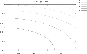
The resulting plot can be viewed in Figure Finite element function on a structured 2D grid: contour plot of the solution. The contour function needs arrays with the \(x\) and \(y\) coordinates expanded to 2D arrays (in the same way as demanded when making vectorized numpy calculations of arithmetic expressions over all grid points). The correctly expanded arrays are stored in grid.coorv. The above call to contour creates 5 equally spaced contour lines, and with clabels='on' the contour values can be seen in the plot.
Other functions for visualizing 2D scalar fields are surf and mesh as known from MATLAB:
import scitools.easyviz as ev
ev.figure()
ev.surf(u_box.grid.coorv[X], u_box.grid.coorv[Y], u_box.values,
        shading='interp', colorbar='on',
        title='surf plot of u', savefig='u_surf.eps')

ev.figure()
ev.mesh(u_box.grid.coorv[X], u_box.grid.coorv[Y], u_box.values,
        title='mesh plot of u', savefig='u_mesh.eps')
Figure Finite element function on a structured 2D grid: surface plot of the solution and Finite element function on a structured 2D grid: lifted mesh plot of the solution exemplify the surfaces arising from the two plotting commands above. You can type pydoc scitools.easyviz in a terminal window to get a full tutorial. Note that scitools.easyviz offers function names like plot and mesh, which clash with plot from dolfin and the mesh variable in our programs. Therefore, we recommend the ev prefix.
A handy feature of BoxMeshField is the ability to give a start point in the grid and a direction, and then extract the field and corresponding coordinates along the nearest grid line. In 3D fields one can also extract data in a plane. Say we want to plot \(u\) along the line \(y=1/2\) in the grid. The grid points, x, and the \(u\) values along this line, uval, are extracted by
start = (0, 0.5)
x, uval, y_fixed, snapped = u_box.gridline(start, direction=X)
The variable snapped is true if the line had to be snapped onto a gridline and in that case y_fixed holds the snapped (altered) \(y\) value. Plotting \(u\) versus the \(x\) coordinate along this line, using scitools.easyviz, is now a matter of
ev.figure()  # new plot window
ev.plot(x, uval, 'r-')  # 'r-: red solid line
ev.title('Solution')
ev.legend('finite element solution')

# or more compactly:
ev.plot(x, uval, 'r-', title='Solution',
        legend='finite element solution')
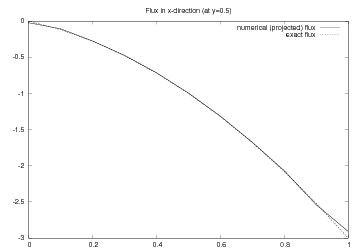
A more exciting plot compares the projected numerical flux in \(x\) direction along the line \(y=1/2\) with the exact flux:
ev.figure()
flux2_x = flux_x if flux_x.ufl_element().degree() == 1 else \
          interpolate(flux_x, FunctionSpace(mesh, 'Lagrange', 1))
flux_x_box = scitools.BoxMeshField.dolfin_function2BoxMeshField(
          flux2_x, mesh, (nx,ny), uniform_mesh=True)
x, fluxval, y_fixed, snapped = \
          flux_x_box.gridline(start, direction=X)
y = y_fixed
flux_x_exact = -(x + y)*2*x
ev.plot(x, fluxval, 'r-',
        x, flux_x_exact, 'b-',
        legend=('numerical (projected) flux', 'exact flux'),
        title='Flux in x-direction (at y=%g)' % y_fixed,
        savefig='flux.eps')
As seen from Figure Finite element function on a structured 2D grid: curve plot of the exact flux and the projected numerical flux, the numerical flux is accurate except in the boundary elements.
The visualization constructions shown above and used to generate the figures are found in the program vcp2D.py in the stationary/poisson directory.
Finite element function on a structured 2D grid: contour plot of the solution
Finite element function on a structured 2D grid: curve plot of the exact flux and the projected numerical flux
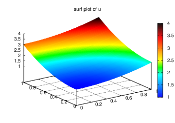
Finite element function on a structured 2D grid: surface plot of the solution
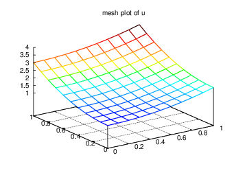
Finite element function on a structured 2D grid: lifted mesh plot of the solution
It should be easy with the information above to transform a finite element field over a uniform rectangular or box-shaped mesh to the corresponding BoxMeshField object and perform MATLAB-style visualizations of the whole field or the field over planes or along lines through the domain. By the transformation to a regular grid we have some more flexibility than what the plot command in DOLFIN offers. However, we remark that comprehensive tools like VisIt, MayaVi2, or ParaView also have the possibility for plotting fields along lines and extracting planes in 3D geometries, though usually with less degree of control compared to Gnuplot, MATLAB, and Matplotlib. For example, in investigations of numerical accuracy or numerical artifacts one is often interested in studying curve plots where only the nodal values sampled. This is straightforward with a structured mesh data structure, but more difficult in visualization packages utilizing unstructured grids, as hitting exactly then nodes when sampling a function along a line through the grid might be non-trivial.
Let us make a slight extension of our two-dimensional Poisson problem from the section The Poisson equation and add a Neumann boundary condition. The domain is still the unit square, but now we set the Dirichlet condition \(u=u_0\) at the left and right sides, \(x=0\) and \(x=1\), while the Neumann condition
is applied to the remaining sides \(y=0\) and \(y=1\). The Neumann condition is also known as a natural boundary condition (in contrast to an essential boundary condition).
Let \(\Gamma_D\) and \(\Gamma_N\) denote the parts of \(\partial\Omega\) where the Dirichlet and Neumann conditions apply, respectively. The complete boundary-value problem can be written as
Again we choose \(u=1+x^2 + 2y^2\) as the exact solution and adjust \(f\), \(g\), and \(u_0\) accordingly:
For ease of programming we may introduce a \(g\) function defined over the whole of \(\Omega\) such that \(g\) takes on the right values at \(y=0\) and \(y=1\). One possible extension is
The first task is to derive the variational problem. This time we cannot omit the boundary term arising from the integration by parts, because \(v\) is only zero on \(\Gamma_D\). We have
and since \(v=0\) on \(\Gamma_D\),
by applying the boundary condition on \(\Gamma_N\). The resulting weak form reads
Expressing this equation in the standard notation \(a(u,v)=L(v)\) is straightforward with
How does the Neumann condition impact the implementation? Starting with any of the previous files d*_p2D.py, say d4_p2D.py, we realize that the statements remain almost the same. Only two adjustments are necessary:
- The function describing the boundary where Dirichlet conditions apply must be modified.
- The new boundary term must be added to the expression in L.
Step 1 can be coded as
def Dirichlet_boundary(x, on_boundary):
    if on_boundary:
        if x[0] == 0 or x[0] == 1:
            return True
        else:
            return False
    else:
        return False
A more compact implementation reads
def Dirichlet_boundary(x, on_boundary):
    return on_boundary and (x[0] == 0 or x[0] == 1)
As pointed out already in the section Implementation (1), testing for an exact match of real numbers is not good programming practice so we introduce a tolerance in the test:
def Dirichlet_boundary(x, on_boundary):
    tol = 1E-14   # tolerance for coordinate comparisons
    return on_boundary and \
           (abs(x[0]) < tol or abs(x[0] - 1) < tol)
The second adjustment of our program concerns the definition of L, where we have to add a boundary integral and a definition of the \(g\) function to be integrated:
g = Expression('-4*x[1]')
L = f*v*dx - g*v*ds
The ds variable implies a boundary integral, while dx implies an integral over the domain \(\Omega\). No more modifications are necessary.
The file dn1_p2D.py in the stationary/poisson directory implements this problem. Running the program verifies the implementation: \(u\) equals the exact solution at all the nodes, regardless of how many elements we use.
The PDE problem from the previous section applies a function \(u_0(x,y)\) for setting Dirichlet conditions at two parts of the boundary. Having a single function to set multiple Dirichlet conditions is seldom possible. The more general case is to have \(m\) functions for setting Dirichlet conditions on \(m\) parts of the boundary. The purpose of this section is to explain how such multiple conditions are treated in FEniCS programs.
Let us return to the case from the section Combining Dirichlet and Neumann Conditions and define two separate functions for the two Dirichlet conditions:
Here, \(\Gamma_0\) is the boundary \(x=0\), while \(\Gamma_1\) corresponds to the boundary \(x=1\). We have that \(u_L = 1 + 2y^2\), \(u_R = 2 + 2y^2\), and \(g=-4y\). For the left boundary \(\Gamma_0\) we define the usual triple of a function for the boundary value, a function for defining the boundary of interest, and a DirichletBC object:
u_L = Expression('1 + 2*x[1]*x[1]')

def left_boundary(x, on_boundary):
    tol = 1E-14   # tolerance for coordinate comparisons
    return on_boundary and abs(x[0]) < tol

Gamma_0 = DirichletBC(V, u_L, left_boundary)
For the boundary \(x=1\) we write a similar code snippet:
u_R = Expression('2 + 2*x[1]*x[1]')

def right_boundary(x, on_boundary):
    tol = 1E-14   # tolerance for coordinate comparisons
    return on_boundary and abs(x[0] - 1) < tol

Gamma_1 = DirichletBC(V, u_R, right_boundary)
The various essential conditions are then collected in a list and used in the solution process:
bcs = [Gamma_0, Gamma_1]
...
solve(a == L, u, bcs)
# or
problem = LinearVariationalProblem(a, L, u, bcs)
solver  = LinearVariationalSolver(problem)
solver.solve()
In other problems, where the \(u\) values are constant at a part of the boundary, we may use a simple Constant object instead of an Expression object.
Debugging of PDE solvers very often faces the question of whether the boundary conditions are set correctly or not. To check which Dirichlet conditions that are actually set in the present problem, we can call the get_boundary_values method in the DirichletBC objects. This method returns a dictionary with degrees of freedom as keys and corresponding essential conditions as values. In the present problem we can write
coor = mesh.coordinates()
for bc in bcs:
    bc_dict = bc.get_boundary_values()
    for dof in bc_dict:
        print 'dof %2d: u=%g\t at point %s' % '
              (dof, bc_dict[dof], str(tuple(coor[dof].tolist())))
The printing of coordinates for each degree of freedom (node here) is only appropriate when degrees of freedom coincide with function values at the vertices of the mesh, which is the case for linear Lagrange elements only. One should therefore make somewhat more robust code that prints out the coordinates (for convenience when checking boundary values) only in the case of first-order Lagrange elements:
Lagrange_1st_order = V.ufl_element().degree() == 1
coor = mesh.coordinates()
for bc in bcs:
    bc_dict = bc.get_boundary_values()
    for dof in bc_dict:
        print 'dof %2d: u=%g' % (dof, bc_dict[dof]),
        if Lagrange_1st_order:  # print vertex coor.
            print '\t at point %s' % \
                  (str(tuple(coor[dof].tolist())))
        else:
            print ''
The output for a mesh made by UnitSquareMesh(3, 2) becomes
dof  0: u=1      at point (0.0, 0.0)
dof  8: u=3      at point (0.0, 1.0)
dof  4: u=1.5    at point (0.0, 0.5)
dof  3: u=2      at point (1.0, 0.0)
dof 11: u=4      at point (1.0, 1.0)
dof  7: u=2.5    at point (1.0, 0.5)
The file dn2_p2D.py contains a complete program which demonstrates the constructions above. An extended example with multiple Neumann conditions would have been quite natural now, but this requires marking various parts of the boundary using the mesh function concept and is therefore left to the section Multiple Neumann, Robin, and Dirichlet Condition.
Given \(a(u,v)=L(v)\), the discrete solution \(u\) is computed by inserting \(u=\sum_{j=1}^N U_j \phi_j\) into \(a(u,v)\) and demanding \(a(u,v)=L(v)\) to be fulfilled for \(N\) test functions \(\hat\phi_1,\ldots,\hat\phi_N\). This implies
which is nothing but a linear system,
where the entries in \(A\) and \(b\) are given by
The examples so far have specified the left- and right-hand side of the variational formulation and then asked FEniCS to assemble the linear system and solve it. An alternative to is explicitly call functions for assembling the coefficient matrix \(A\) and the right-side vector \(b\), and then solve the linear system \(AU=b\) with respect to the \(U\) vector. Instead of solve(a == L, u, b) we now write
A = assemble(a)
b = assemble(L)
bc.apply(A, b)
u = Function(V)
U = u.vector()
solve(A, U, b)
The variables a and L are as before. That is, a refers to the bilinear form involving a TrialFunction object (say u) and a TestFunction object (v), and L involves a TestFunction object (v). From a and L, the assemble function can compute \(A\) and \(b\).
The matrix \(A\) and vector \(b\) are first assembled without incorporating essential (Dirichlet) boundary conditions. Thereafter, the call bc.apply(A, b) performs the necessary modifications of the linear system such that u is guaranteed to equal the prescribed boundary values. When we have multiple Dirichlet conditions stored in a list bcs, as explained in the section Multiple Dirichlet Conditions, we must apply each condition in bcs to the system:
# bcs is a list of DirichletBC objects
for bc in bcs:
    bc.apply(A, b)
There is an alternative function assemble_system, which can assemble the system and take boundary conditions into account in one call:
A, b = assemble_system(a, L, bcs)
The assemble_system function incorporates the boundary conditions in the element matrices and vectors, prior to assembly. The conditions are also incorporated in a symmetric way to preserve eventual symmetry of the coefficient matrix.
With bc.apply(A, b) the matrix A is modified in an unsymmetric way.
Note that the solution u is, as before, a Function object. The degrees of freedom, \(U=A^{-1}b\), are filled into u‘s Vector object (u.vector()) by the solve function.
The object A is of type Matrix, while b and u.vector() are of type Vector. We may convert the matrix and vector data to numpy arrays by calling the array() method as shown before. If you wonder how essential boundary conditions are incorporated in the linear system, you can print out A and b before and after the bc.apply(A, b) call:
A = assemble(a)
b = assemble(L)
if mesh.num_cells() < 16:  # print for small meshes only
    print A.array()
    print b.array()
bc.apply(A, b)
if mesh.num_cells() < 16:
    print A.array()
    print b.array()
With access to the elements in A through a numpy array we can easily perform computations on this matrix, such as computing the eigenvalues (using the eig function in numpy.linalg). We can alternatively dump A.array() and b.array() to file in MATLAB format and invoke MATLAB or Octave to analyze the linear system. Dumping the arrays to MATLAB format is done by
import scipy.io
scipy.io.savemat('Ab.mat', {'A': A.array(), 'b': b.array()})
Writing load Ab.mat in MATLAB or Octave will then make the array variables A and b available for computations.
Matrix processing in Python or MATLAB/Octave is only feasible for small PDE problems since the numpy arrays or matrices in MATLAB file format are dense matrices. DOLFIN also has an interface to the eigensolver package SLEPc, which is a preferred tool for computing the eigenvalues of large, sparse matrices of the type encountered in PDE problems (see demo/la/eigenvalue in the DOLFIN source code tree for a demo).
A complete code where the linear system \(AU=b\) is explicitly assembled and solved is found in the file dn3_p2D.py in the directory stationary/poisson. This code solves the same problem as in dn2_p2D.py (the section Multiple Dirichlet Conditions). For small linear systems, the program writes out A and b before and after incorporation of essential boundary conditions and illustrates the difference between assemble and assemble_system. The reader is encouraged to run the code for a \(2\times 1\) mesh (UnitSquareMesh(2, 1) and study the output of A.
By default, solve(A, U, b) applies sparse LU decomposition as solver. Specification of an iterative solver and preconditioner is done through two optional arguments:
solve(A, U, b, 'cg', 'ilu')
Appropriate names of solvers and preconditioners are found in the section Linear Solvers and Preconditioners.
To control tolerances in the stopping criterion and the maximum number of iterations, one can explicitly form a KrylovSolver object and set items in its parameters attribute (see also the section Linear Variational Problem and Solver Objects):
solver = KrylovSolver('cg', 'ilu')
solver.parameters['absolute_tolerance'] = 1E-7
solver.parameters['relative_tolerance'] = 1E-4
solver.parameters['maximum_iterations'] = 1000
u = Function(V)
U = u.vector()
set_log_level(DEBUG)
solver.solve(A, U, b)
The program dn4_p2D.py is a modification of dn3_p2D.py illustrating this latter approach.
The choice of start vector for the iterations in a linear solver is often important. With the solver.solve(A, U, b) call the default start vector is the zero vector. A start vector with random numbers in the interval \([-100,100]\) can be computed as
n = u.vector().array().size
U = u.vector()
U[:] = numpy.random.uniform(-100, 100, n)
solver.parameters['nonzero_initial_guess'] = True
solver.solve(A, U, b)
Note that we must turn off the default behavior of setting the start vector (“initial guess”) to zero. A random start vector is included in the dn4_p2D.py code.
Creating the linear system explicitly in a program can have some advantages in more advanced problem settings. For example, \(A\) may be constant throughout a time-dependent simulation, so we can avoid recalculating \(A\) at every time level and save a significant amount of simulation time. The sections Implementation (2) and Avoiding Assembly deal with this topic in detail.
FEniCS makes it is easy to write a unified simulation code that can operate in 1D, 2D, and 3D. We will conveniently make use of this feature in forthcoming examples. As an appetizer, go back to the introductory program d1_p2D.py in the stationary/poisson directory and change the mesh construction from UnitSquareMesh(6, 4) to UnitCubeMesh(6, 4, 5). Now the domain is the unit cube partitioned into \(6\times 4\times 5\) boxes, and each box is divided into six tetrahedra-shaped finite elements for computations. Run the program and observe that we can solve a 3D problem without any other modifications (!). The visualization allows you to rotate the cube and observe the function values as colors on the boundary.
The forthcoming material introduces some convenient technicalities such that the same program can run in 1D, 2D, or 3D without any modifications. Consider the simple model problem
with exact solution \(u(x)=x^2\). Our aim is to formulate and solve this problem in a 2D and a 3D domain as well. We may generalize the domain \([0,1]\) to a rectangle or box of any size in the \(y\) and \(z\) directions and pose homogeneous Neumann conditions \(\partial u/\partial n = 0\) at all additional boundaries \(y=\mbox{const}\) and \(z=\mbox{const}\) to ensure that \(u\) only varies with \(x\). For example, let us choose a unit hypercube as domain: \(\Omega = [0,1]^d\), where \(d\) is the number of space dimensions. The generalized \(d\)-dimensional Poisson problem then reads
where \(\Gamma_0\) is the side of the hypercube where \(x=0\), and where \(\Gamma_1\) is the side where \(x=1\).
Implementing a PDE for any \(d\) is no more complicated than solving a problem with a specific number of dimensions. The only non-trivial part of the code is actually to define the mesh. We use the command line for the user-input to the program. The first argument can be the degree of the polynomial in the finite element basis functions. Thereafter, we supply the cell divisions in the various spatial directions. The number of command-line arguments will then imply the number of space dimensions. For example, writing 3 10 3 4 on the command line means that we want to approximate \(u\) by piecewise polynomials of degree 3, and that the domain is a three-dimensional cube with \(10\times 3\times 4\) divisions in the \(x\), \(y\), and \(z\) directions, respectively.
The Python code can be quite compact:
degree = int(sys.argv[1])
divisions = [int(arg) for arg in sys.argv[2:]]
d = len(divisions)
domain_type = [UnitIntervalMesh, UnitSquareMesh, UnitCubeMesh]
mesh = domain_type[d-1](*divisions)
V = FunctionSpace(mesh, 'Lagrange', degree)
First note that although sys.argv[2:] holds the divisions of the mesh, all elements of the list sys.argv[2:] are string objects, so we need to explicitly convert each element to an integer. The construction domain_type[d-1] will pick the right name of the object used to define the domain and generate the mesh. Moreover, the argument *divisions sends all the component of the list divisions as separate arguments. For example, in a 2D problem where divisions has two elements, the statement
mesh = domain_type[d-1](*divisions)
is equivalent to
mesh = UnitSquareMesh(divisions[0], divisions[1])
The next part of the program is to set up the boundary conditions. Since the Neumann conditions have \(\partial u/\partial n=0\) we can omit the boundary integral from the weak form. We then only need to take care of Dirichlet conditions at two sides:
tol = 1E-14   # tolerance for coordinate comparisons
def Dirichlet_boundary0(x, on_boundary):
    return on_boundary and abs(x[0]) < tol

def Dirichlet_boundary1(x, on_boundary):
    return on_boundary and abs(x[0] - 1) < tol

bc0 = DirichletBC(V, Constant(0), Dirichlet_boundary0)
bc1 = DirichletBC(V, Constant(1), Dirichlet_boundary1)
bcs = [bc0, bc1]
Note that this code is independent of the number of space dimensions. So are the statements defining and solving the variational problem:
u = TrialFunction(V)
v = TestFunction(V)
f = Constant(-2)
a = inner(nabla_grad(u), nabla_grad(v))*dx
L = f*v*dx

u = Function(V)
solve(a == L, u, bcs)
The complete code is found in the file paD.py (Poisson problem in “anyD”).
If we want to parameterize the direction in which \(u\) varies, say by the space direction number e, we only need to replace x[0] in the code by x[e]. The parameter e could be given as a second command-line argument. The reader is encouraged to perform this modification.
Now we shall address how to solve nonlinear PDEs in FEniCS. Our sample PDE for implementation is taken as a nonlinear Poisson equation:
The coefficient \(q(u)\) makes the equation nonlinear (unless \(q(u)\) is constant in \(u\)).
To be able to easily verify our implementation, we choose the domain, \(q(u)\), \(f\), and the boundary conditions such that we have a simple, exact solution \(u\). Let \(\Omega\) be the unit hypercube \([0, 1]^d\) in \(d\) dimensions, \(q(u)=(1+u)^m\), \(f=0\), \(u=0\) for \(x_0=0\), \(u=1\) for \(x_0=1\), and \(\partial u/\partial n=0\) at all other boundaries \(x_i=0\) and \(x_i=1\), \(i=1,\ldots,d-1\). The coordinates are now represented by the symbols \(x_0,\ldots,x_{d-1}\). The exact solution is then
We refer to the section Parameterizing the Number of Space Dimensions for details on formulating a PDE problem in \(d\) space dimensions.
The variational formulation of our model problem reads: Find \(u \in V\) such that
where
and
The discrete problem arises as usual by restricting \(V\) and \(\hat V\) to a pair of discrete spaces. As usual, we omit any subscript on discrete spaces and simply say \(V\) and \(\hat V\) are chosen finite dimensional according to some mesh with some element type. Similarly, we let \(u\) be the discrete solution and use \(u_{\mbox{e}}\) for the exact solution if it becomes necessary to distinguish between the two.
The discrete nonlinear problem is then wirtten as: find \(u\in V\) such that
with \(u = \sum_{j=1}^N U_j \phi_j\). Since \(F\) is a nonlinear function of \(u\), the variational statement gives rise to a system of nonlinear algebraic equations.
FEniCS can be used in alternative ways for solving a nonlinear PDE problem. We shall in the following subsections go through four solution strategies:
- a simple Picard-type iteration,
- a Newton method at the algebraic level,
- a Newton method at the PDE level, and
- an automatic approach where FEniCS attacks the nonlinear variational problem directly.
The “black box” strategy 4 is definitely the simplest one from a programmer’s point of view, but the others give more manual control of the solution process for nonlinear equations (which also has some pedagogical advantages, especially for newcomers to nonlinear finite element problems).
Picard iteration is an easy way of handling nonlinear PDEs: we simply use a known, previous solution in the nonlinear terms so that these terms become linear in the unknown \(u\). The strategy is also known as the method of successive substitutions. For our particular problem, we use a known, previous solution in the coefficient \(q(u)\). More precisely, given a solution \(u^k\) from iteration \(k\), we seek a new (hopefully improved) solution \(u^{k+1}\) in iteration \(k+1\) such that \(u^{k+1}\) solves the linear problem,
The iterations require an initial guess \(u^0\). The hope is that \(u^{k} \rightarrow u\) as \(k\rightarrow\infty\), and that \(u^{k+1}\) is sufficiently close to the exact solution \(u\) of the discrete problem after just a few iterations.
We can easily formulate a variational problem for \(u^{k+1}\) from the last equation. Equivalently, we can approximate \(q(u)\) by \(q(u^k)\) in \(\int_\Omega q(u)\nabla u\cdot \nabla v {\, \mathrm{d}x}\) to obtain the same linear variational problem. In both cases, the problem consists of seeking \(u^{k+1} \in V\) such that
with
Since this is a linear problem in the unknown \(u^{k+1}\), we can equivalently use the formulation
with
The iterations can be stopped when \(\epsilon\equiv ||u^{k+1}-u^k|| < \mbox{tol}\), where \(\mbox{tol}\) is a small tolerance, say \(10^{-5}\), or when the number of iterations exceed some critical limit. The latter case will pick up divergence of the method or unacceptable slow convergence.
In the solution algorithm we only need to store \(u^k\) and \(u^{k+1}\), called u_k and u in the code below. The algorithm can then be expressed as follows:
def q(u):
    return (1+u)**m

# Define variational problem for Picard iteration
u = TrialFunction(V)
v = TestFunction(V)
u_k = interpolate(Constant(0.0), V)  # previous (known) u
a = inner(q(u_k)*nabla_grad(u), nabla_grad(v))*dx
f = Constant(0.0)
L = f*v*dx

# Picard iterations
u = Function(V)     # new unknown function
eps = 1.0           # error measure ||u-u_k||
tol = 1.0E-5        # tolerance
iter = 0            # iteration counter
maxiter = 25        # max no of iterations allowed
while eps > tol and iter < maxiter:
    iter += 1
    solve(a == L, u, bcs)
    diff = u.vector().array() - u_k.vector().array()
    eps = numpy.linalg.norm(diff, ord=numpy.Inf)
    print 'iter=%d: norm=%g' % (iter, eps)
    u_k.assign(u)   # update for next iteration
We need to define the previous solution in the iterations, u_k, as a finite element function so that u_k can be updated with u at the end of the loop. We may create the initial Function u_k by interpolating an Expression or a Constant to the same vector space as u lives in (V).
In the code above we demonstrate how to use numpy functionality to compute the norm of the difference between the two most recent solutions. Here we apply the maximum norm (\(\ell_\infty\) norm) on the difference of the solution vectors (ord=1 and ord=2 give the \(\ell_1\) and \(\ell_2\) vector norms - other norms are possible for numpy arrays, see pydoc numpy.linalg.norm).
The file picard_np.py contains the complete code for this nonlinear Poisson problem. The implementation is \(d\) dimensional, with mesh construction and setting of Dirichlet conditions as explained in the section Parameterizing the Number of Space Dimensions. For a \(33\times 33\) grid with \(m=2\) we need 9 iterations for convergence when the tolerance is \(10^{-5}\).
After having discretized our nonlinear PDE problem, we may use Newton’s method to solve the system of nonlinear algebraic equations. From the continuous variational problem, the discrete version results in a system of equations for the unknown parameters \(U_1,\ldots, U_N\)
Newton’s method for the system \(F_i(U_1,\ldots,U_j)=0\), \(i=1,\ldots,N\) can be formulated as
where \(\omega\in [0,1]\) is a relaxation parameter, and \(k\) is an iteration index. An initial guess \(u^0\) must be provided to start the algorithm.
The original Newton method has \(\omega=1\), but in problems where it is difficult to obtain convergence, so-called under-relaxation with \(\omega < 1\) may help. It means that one takes a smaller step than what is suggested by Newton’s method.
We need, in a program, to compute the Jacobian matrix \(\partial F_i/\partial U_j\) and the right-hand side vector \(-F_i\). Our present problem has \(F_i\) given by above. The derivative \(\partial F_i/\partial U_j\) becomes
The following results were used to obtain the previous equation:
We can reformulate the Jacobian matrix by introducing the short notation \(u^k = \sum_{j=1}^NU_j^k\phi_j\):
In order to make FEniCS compute this matrix, we need to formulate a corresponding variational problem. Looking at the linear system of equations in Newton’s method,
we can introduce \(v\) as a general test function replacing \(\hat\phi_i\), and we can identify the unknown \(\delta u = \sum_{j=1}^N\delta U_j\phi_j\). From the linear system we can now go “backwards” to construct the corresponding linear discrete weak form to be solved in each Newton iteration:
This variational form fits the standard notation \(a(\delta u,v)=L(v)\) with
Note the important feature in Newton’s method that the previous solution \(u^k\) replaces \(u\) in the formulas when computing the matrix \(\partial F_i/\partial U_j\) and vector \(F_i\) for the linear system in each Newton iteration.
We now turn to the implementation. To obtain a good initial guess \(u^0\), we can solve a simplified, linear problem, typically with \(q(u)=1\), which yields the standard Laplace equation \(\nabla^2 u^0 =0\). The recipe for solving this problem appears in the sections Variational Formulation, Implementation (1), and Combining Dirichlet and Neumann Conditions. The code for computing \(u^0\) becomes as follows:
tol = 1E-14
def left_boundary(x, on_boundary):
    return on_boundary and abs(x[0]) < tol

def right_boundary(x, on_boundary):
    return on_boundary and abs(x[0]-1) < tol

Gamma_0 = DirichletBC(V, Constant(0.0), left_boundary)
Gamma_1 = DirichletBC(V, Constant(1.0), right_boundary)
bcs = [Gamma_0, Gamma_1]

# Define variational problem for initial guess (q(u)=1, i.e., m=0)
u = TrialFunction(V)
v = TestFunction(V)
a = inner(nabla_grad(u), nabla_grad(v))*dx
f = Constant(0.0)
L = f*v*dx
A, b = assemble_system(a, L, bcs)
u_k = Function(V)
U_k = u_k.vector()
solve(A, U_k, b)
Here, u_k denotes the solution function for the previous iteration, so that the solution after each Newton iteration is u = u_k + omega*du. Initially, u_k is the initial guess we call \(u^0\) in the mathematics.
The Dirichlet boundary conditions for \(\delta u\), in the problem to be solved in each Newton iteration, are somewhat different than the conditions for \(u\). Assuming that \(u^k\) fulfills the Dirichlet conditions for \(u\), \(\delta u\) must be zero at the boundaries where the Dirichlet conditions apply, in order for \(u^{k+1}=u^k + \omega\delta u\) to fulfill the right boundary values. We therefore define an additional list of Dirichlet boundary conditions objects for \(\delta u\):
Gamma_0_du = DirichletBC(V, Constant(0), left_boundary)
Gamma_1_du = DirichletBC(V, Constant(0), right_boundary)
bcs_du = [Gamma_0_du, Gamma_1_du]
The nonlinear coefficient and its derivative must be defined before coding the weak form of the Newton system:
def q(u):
    return (1+u)**m

def Dq(u):
    return m*(1+u)**(m-1)

du = TrialFunction(V) # u = u_k + omega*du
a = inner(q(u_k)*nabla_grad(du), nabla_grad(v))*dx + \
    inner(Dq(u_k)*du*nabla_grad(u_k), nabla_grad(v))*dx
L = -inner(q(u_k)*nabla_grad(u_k), nabla_grad(v))*dx
The Newton iteration loop is very similar to the Picard iteration loop in the section Picard Iteration:
du = Function(V)
u  = Function(V)  # u = u_k + omega*du
omega = 1.0       # relaxation parameter
eps = 1.0
tol = 1.0E-5
iter = 0
maxiter = 25
while eps > tol and iter < maxiter:
    iter += 1
    A, b = assemble_system(a, L, bcs_du)
    solve(A, du.vector(), b)
    eps = numpy.linalg.norm(du.vector().array(), ord=numpy.Inf)
    print 'Norm:', eps
    u.vector()[:] = u_k.vector() + omega*du.vector()
    u_k.assign(u)
There are other ways of implementing the update of the solution as well:
u.assign(u_k)  # u = u_k
u.vector().axpy(omega, du.vector())

# or
u.vector()[:] += omega*du.vector()
The axpy(a, y) operation adds a scalar a times a Vector y to a Vector object. It is usually a fast operation calling up an optimized BLAS routine for the calculation.
Mesh construction for a \(d\)-dimensional problem with arbitrary degree of the Lagrange elements can be done as explained in the section Parameterizing the Number of Space Dimensions. The complete program appears in the file alg_newton_np.py.
Although Newton’s method in PDE problems is normally formulated at the linear algebra level, i.e., as a solution method for systems of nonlinear algebraic equations, we can also formulate the method at the PDE level. This approach yields a linearization of the PDEs before they are discretized. FEniCS users will probably find this technique simpler to apply than the more standard method in the section A Newton Method at the Algebraic Level.
Given an approximation to the solution field, \(u^k\), we seek a perturbation \(\delta u\) so that
fulfills the nonlinear PDE. However, the problem for \(\delta u\) is still nonlinear and nothing is gained. The idea is therefore to assume that \(\delta u\) is sufficiently small so that we can linearize the problem with respect to \(\delta u\). Inserting \(u^{k+1}\) in the PDE, linearizing the \(q\) term as
and dropping nonlinear terms in \(\delta u\), we get
We may collect the terms with the unknown \(\delta u\) on the left-hand side,
The weak form of this PDE is derived by multiplying by a test function \(v\) and integrating over \(\Omega\), integrating as usual the second-order derivatives by parts:
The variational problem reads: find \(\delta u\in V\) such that \(a(\delta u,v) = L(v)\) for all \(v\in \hat V\), where
The function spaces \(V\) and \(\hat V\), being continuous or discrete, are as in the linear Poisson problem from the section Variational Formulation.
We must provide some initial guess, e.g., the solution of the PDE with \(q(u)=1\). The corresponding weak form \(a_0(u^0,v)=L_0(v)\) has
Thereafter, we enter a loop and solve \(a(\delta u,v)=L(v)\) for \(\delta u\) and compute a new approximation \(u^{k+1} = u^k + \delta u\). Note that \(\delta u\) is a correction, so if \(u^0\) satisfies the prescribed Dirichlet conditions on some part \(\Gamma_D\) of the boundary, we must demand \(\delta u=0\) on \(\Gamma_D\).
Looking at the equations just derived, we see that the variational form is the same as for the Newton method at the algebraic level in the section A Newton Method at the Algebraic Level. Since Newton’s method at the algebraic level required some “backward” construction of the underlying weak forms, FEniCS users may prefer Newton’s method at the PDE level, which this author finds more straightforward, although not so commonly documented in the literature on numerical methods for PDEs. There is seemingly no need for differentiations to derive a Jacobian matrix, but a mathematically equivalent derivation is done when nonlinear terms are linearized using the first two Taylor series terms and when products in the perturbation \(\delta u\) are neglected.
The implementation is identical to the one in the section A Newton Method at the Algebraic Level and is found in the file pde_newton_np.py. The reader is encouraged to go through this code to be convinced that the present method actually ends up with the same program as needed for the Newton method at the linear algebra level in the section A Newton Method at the Algebraic Level.
The previous hand-calculations and manual implementation of Picard or Newton methods can be automated by tools in FEniCS. In a nutshell, one can just write
problem = NonlinearVariationalProblem(F, u, bcs, J)
solver  = NonlinearVariationalSolver(problem)
solver.solve()
where F corresponds to the nonlinear form \(F(u;v)\), u is the unknown Function object, bcs represents the essential boundary conditions (in general a list of DirichletBC objects), and J is a variational form for the Jacobian of F.
Let us explain in detail how to use the built-in tools for nonlinear variational problems and their solution. The appropriate F form is straightforwardly defined as follows, assuming q(u) is coded as a Python function:
u_ = Function(V)     # most recently computed solution
v  = TestFunction(V)
F  = inner(q(u_)*nabla_grad(u_), nabla_grad(v))*dx
Note here that u_ is a Function (not a TrialFunction). An alternative and perhaps more intuitive formula for \(F\) is to define \(F(u;v)\) directly in terms of a trial function for \(u\) and a test function for \(v\), and then create the proper F by
u  = TrialFunction(V)
v  = TestFunction(V)
F  = inner(q(u)*nabla_grad(u), nabla_grad(v))*dx
u_ = Function(V)     # the most recently computed solution
F  = action(F, u_)
The latter statement is equivalent to \(F(u=u_{-}; v)\), where \(u_{-}\) is an existing finite element function representing the most recently computed approximation to the solution. (Note that \(u^k\) and \(u^{k+1}\) in the previous notation correspond to \(u_{-}\) and \(u\) in the present notation. We have changed notation to better align the mathematics with the associated UFL code.)
The derivative \(J\) (J) of \(F\) (F) is formally the Gateaux derivative \(DF(u^k; \delta u, v)\) of \(F(u;v)\) at \(u=u_{-}\) in the direction of \(\delta u\). Technically, this Gateaux derivative is derived by computing
The \(\delta u\) is now the trial function and \(u_{-}\) is the previous approximation to the solution \(u\). We start with
and obtain
which leads to
as \(\epsilon\rightarrow 0\). This last expression is the Gateaux derivative of \(F\). We may use \(J\) or \(a(\delta u, v)\) for this derivative, the latter having the advantage that we easily recognize the expression as a bilinear form. However, in the forthcoming code examples J is used as variable name for the Jacobian.
The specification of J goes as follows if du is the TrialFunction:
du = TrialFunction(V)
v  = TestFunction(V)
u_ = Function(V)      # the most recently computed solution
F  = inner(q(u_)*nabla_grad(u_), nabla_grad(v))*dx

J = inner(q(u_)*nabla_grad(du), nabla_grad(v))*dx + \
    inner(Dq(u_)*du*nabla_grad(u_), nabla_grad(v))*dx
The alternative specification of F, with u as TrialFunction, leads to
u  = TrialFunction(V)
v  = TestFunction(V)
u_ = Function(V)      # the most recently computed solution
F  = inner(q(u)*nabla_grad(u), nabla_grad(v))*dx
F  = action(F, u_)

J = inner(q(u_)*nabla_grad(u), nabla_grad(v))*dx + \
    inner(Dq(u_)*u*nabla_grad(u_), nabla_grad(v))*dx
The UFL language, used to specify weak forms, supports differentiation of forms. This feature facilitates automatic symbolic computation of the Jacobian J by calling the function derivative with F, the most recently computed solution (Function), and the unknown (TrialFunction) as parameters:
du = TrialFunction(V)
v  = TestFunction(V)
u_ = Function(V)      # the most recently computed solution
F  = inner(q(u_)*nabla_grad(u_), nabla_grad(v))*dx

J  = derivative(F, u_, du)  # Gateaux derivative in dir. of du
or
u  = TrialFunction(V)
v  = TestFunction(V)
u_ = Function(V)      # the most recently computed solution
F  = inner(q(u)*nabla_grad(u), nabla_grad(v))*dx
F  = action(F, u_)

J  = derivative(F, u_, u)   # Gateaux derivative in dir. of u
The derivative function is obviously very convenient in problems where differentiating F by hand implies lengthy calculations.
The preferred implementation of F and J, depending on whether du or u is the TrialFunction object, is a matter of personal taste. Derivation of the Gateaux derivative by hand, as shown above, is most naturally matched by an implementation where du is the TrialFunction, while use of automatic symbolic differentiation with the aid of the derivative function is most naturally matched by an implementation where u is the TrialFunction. We have implemented both approaches in two files: vp1_np.py with u as TrialFunction, and vp2_np.py with du as TrialFunction. The directory stationary/nonlinear_poisson contains both files. The first command-line argument determines if the Jacobian is to be automatically derived or computed from the hand-derived formula.
The following code defines the nonlinear variational problem and an associated solver based on Newton’s method. We here demonstrate how key parameters in Newton’s method can be set, as well as the choice of solver and preconditioner, and associated parameters, for the linear system occurring in the Newton iteration.
problem = NonlinearVariationalProblem(F, u_, bcs, J)
solver  = NonlinearVariationalSolver(problem)

prm = solver.parameters
prm['newton_solver']['absolute_tolerance'] = 1E-8
prm['newton_solver']['relative_tolerance'] = 1E-7
prm['newton_solver']['maximum_iterations'] = 25
prm['newton_solver']['relaxation_parameter'] = 1.0
if iterative_solver:
    prm['linear_solver'] = 'gmres'
    prm['preconditioner'] = 'ilu'
    prm['krylov_solver']['absolute_tolerance'] = 1E-9
    prm['krylov_solver']['relative_tolerance'] = 1E-7
    prm['krylov_solver']['maximum_iterations'] = 1000
    prm['krylov_solver']['gmres']['restart'] = 40
    prm['krylov_solver']['preconditioner']['ilu']['fill_level'] = 0
set_log_level(PROGRESS)

solver.solve()
A list of available parameters and their default values can as usual be printed by calling info(prm, True). The u_ we feed to the nonlinear variational problem object is filled with the solution by the call solver.solve().
The examples in the section Fundamentals illustrate that solving linear, stationary PDE problems with the aid of FEniCS is easy and requires little programming. That is, FEniCS automates the spatial discretization by the finite element method. The solution of nonlinear problems, as we showed in the section Nonlinear Problems, can also be automated (cf. The section Solving the Nonlinear Variational Problem Directly), but many scientists will prefer to code the solution strategy of the nonlinear problem themselves and experiment with various combinations of strategies in difficult problems. Time-dependent problems are somewhat similar in this respect: we have to add a time discretization scheme, which is often quite simple, making it natural to explicitly code the details of the scheme so that the programmer has full control. We shall explain how easily this is accomplished through examples.
Our time-dependent model problem for teaching purposes is naturally the simplest extension of the Poisson problem into the time domain, i.e., the diffusion problem
Here, \(u\) varies with space and time, e.g., \(u=u(x,y,t)\) if the spatial domain \(\Omega\) is two-dimensional. The source function \(f\) and the boundary values \(u_0\) may also vary with space and time. The initial condition \(I\) is a function of space only.
A straightforward approach to solving time-dependent PDEs by the finite element method is to first discretize the time derivative by a finite difference approximation, which yields a recursive set of stationary problems, and then turn each stationary problem into a variational formulation.
Let superscript \(k\) denote a quantity at time \(t_k\), where \(k\) is an integer counting time levels. For example, \(u^k\) means \(u\) at time level \(k\). A finite difference discretization in time first consists in sampling the PDE at some time level, say \(k\):
The time-derivative can be approximated by a finite difference. For simplicity and stability reasons we choose a simple backward difference:
where \({{\Delta t}}\) is the time discretization parameter. Inserting this approximation in the PDE yields
This is our time-discrete version of the diffusion PDE problem. Reordering the last equation so that \(u^k\) appears on the left-hand side only, yields a recursive set of spatial (stationary) problems for \(u^k\) (assuming \(u^{k-1}\) is known from computations at the previous time level):
Given \(I\), we can solve for \(u^0\), \(u^1\), \(u^2\), and so on.
We use a finite element method to solve the time-discrete equations which still have spatial differential operators. This requires turning the equations into weak forms. As usual, we multiply by a test function \(v\in \hat V\) and integrate second-derivatives by parts. Introducing the symbol \(u\) for \(u^k\) (which is natural in the program too), the resulting weak form can be conveniently written in the standard notation: \(a_0(u,v)=L_0(v)\) for the initial step and \(a(u,v)=L(v)\) for a general step, where
The continuous variational problem is to find \(u^0\in V\) such that \(a_0(u^0,v)=L_0(v)\) holds for all \(v\in\hat V\), and then find \(u^k\in V\) such that \(a(u^k,v)=L(v)\) for all \(v\in\hat V\), \(k=1,2,\ldots\).
Approximate solutions in space are found by restricting the functional spaces \(V\) and \(\hat V\) to finite-dimensional spaces, exactly as we have done in the Poisson problems. We shall use the symbol \(u\) for the finite element approximation at time \(t_k\). In case we need to distinguish this space-time discrete approximation from the exact solution of the continuous diffusion problem, we use \(u_{\mbox{e}}\) for the latter. By \(u^{k-1}\) we mean, from now on, the finite element approximation of the solution at time \(t_{k-1}\).
Note that the forms \(a_0\) and \(L_0\) are identical to the forms met in the section Computing Derivatives, except that the test and trial functions are now scalar fields and not vector fields. Instead of solving an equation for \(u^0\) by a finite element method, i.e., projecting \(I\) onto \(V\) via the problem \(a_0(u,v)=L_0(v)\), we could simply interpolate \(u^0\) from \(I\). That is, if \(u^0=\sum_{j=1}^N U^0_j\phi_j\), we simply set \(U_j=I(x_j,y_j)\), where \((x_j,y_j)\) are the coordinates of node number \(j\). We refer to these two strategies as computing the initial condition by either projecting \(I\) or interpolating \(I\). Both operations are easy to compute through one statement, using either the project or interpolate function.
Our program needs to perform the time stepping explicitly, but can rely on FEniCS to easily compute \(a_0\), \(L_0\), \(a\), and \(L\), and solve the linear systems for the unknowns. We realize that \(a\) does not depend on time, which means that its associated matrix also will be time independent. Therefore, it is wise to explicitly create matrices and vectors as in the section A Linear Algebra Formulation. The matrix \(A\) arising from \(a\) can be computed prior to the time stepping, so that we only need to compute the right-hand side \(b\), corresponding to \(L\), in each pass in the time loop. Let us express the solution procedure in algorithmic form, writing \(u\) for the unknown spatial function at the new time level (\(u^k\)) and \(u_1\) for the spatial solution at one earlier time level (\(u^{k-1}\)):
- define Dirichlet boundary condition (\(u_0\), Dirichlet boundary, etc.)
- if \(u_1\) is to be computed by projecting \(I\):
- define \(a_0\) and \(L_0\)
- assemble matrix \(M\) from \(a_0\) and vector \(b\) from \(L_0\)
- solve \(MU=b\) and store \(U\) in \(u_1\)
- else: (interpolation)
- let \(u_1\) interpolate \(I\)
- define \(a\) and \(L\)
- assemble matrix \(A\) from \(a\)
- set some stopping time \(T\)
- \(t={{\Delta t}}\)
- while \(t\leq T\)
- assemble vector \(b\) from \(L\)
- apply essential boundary conditions
- solve \(AU=b\) for \(U\) and store in \(u\)
- \(t\leftarrow t + {{\Delta t}}\)
- \(u_1 \leftarrow u\) (be ready for next step)
Before starting the coding, we shall construct a problem where it is easy to determine if the calculations are correct. The simple backward time difference is exact for linear functions, so we decide to have a linear variation in time. Combining a second-degree polynomial in space with a linear term in time,
yields a function whose computed values at the nodes may be exact, regardless of the size of the elements and \({{\Delta t}}\), as long as the mesh is uniformly partitioned. We realize by inserting the simple solution in the PDE problem that \(u_0\) must be given as (?) and that \(f(x,y,t)=\beta - 2 - 2\alpha\) and \(I(x,y)=1+x^2+\alpha y^2\).
A new programming issue is how to deal with functions that vary in space and time, such as the the boundary condition \(u_0\). A natural solution is to apply an Expression object with time \(t\) as a parameter, in addition to the parameters \(\alpha\) and \(\beta\) (see the section Solving a Real Physical Problem for Expression objects with parameters):
alpha = 3; beta = 1.2
u0 = Expression('1 + x[0]*x[0] + alpha*x[1]*x[1] + beta*t',
                alpha=alpha, beta=beta, t=0)
The time parameter can later be updated by assigning values to u0.t.
Given a mesh and an associated function space V, we can specify the \(u_0\) function as
alpha = 3; beta = 1.2
u0 = Expression('1 + x[0]*x[0] + alpha*x[1]*x[1] + beta*t',
                {'alpha': alpha, 'beta': beta})
u0.t = 0
This function expression has the components of x as independent variables, while alpha, beta, and t are parameters. The parameters can either be set through a dictionary at construction time, as demonstrated for alpha and beta, or anytime through attributes in the function object, as shown for the t parameter.
The essential boundary conditions, along the whole boundary in this case, are set in the usual way,
def boundary(x, on_boundary):  # define the Dirichlet boundary
    return on_boundary

bc = DirichletBC(V, u0, boundary)
We shall use u for the unknown \(u\) at the new time level and u_1 for \(u\) at the previous time level. The initial value of u_1, implied by the initial condition on \(u\), can be computed by either projecting or interpolating \(I\). The \(I(x,y)\) function is available in the program through u0, as long as u0.t is zero. We can then do
u_1 = interpolate(u0, V)
# or
u_1 = project(u0, V)
Note that we could, as an equivalent alternative to using project, define \(a_0\) and \(L_0\) as we did in the section Computing Derivatives and form the associated variational problem. To actually recover the exact solution to machine precision, it is important not to compute the discrete initial condition by projecting \(I\), but by interpolating \(I\) so that the nodal values are exact at \(t=0\) (projection results in approximative values at the nodes).
The definition of \(a\) and \(L\) goes as follows:
dt = 0.3      # time step

u = TrialFunction(V)
v = TestFunction(V)
f = Constant(beta - 2 - 2*alpha)

a = u*v*dx + dt*inner(nabla_grad(u), nabla_grad(v))*dx
L = (u_1 + dt*f)*v*dx

A = assemble(a)   # assemble only once, before the time stepping
Finally, we perform the time stepping in a loop:
u = Function(V)   # the unknown at a new time level
T = 2             # total simulation time
t = dt

while t <= T:
    b = assemble(L)
    u0.t = t
    bc.apply(A, b)
    solve(A, u.vector(), b)

    t += dt
    u_1.assign(u)
Observe that u0.t must be updated before the bc.apply statement, to enforce computation of Dirichlet conditions at the current time level.
The time loop above does not contain any comparison of the numerical and the exact solution, which we must include in order to verify the implementation. As in many previous examples, we compute the difference between the array of nodal values of u and the array of the interpolated exact solution. The following code is to be included inside the loop, after u is found:
u_e = interpolate(u0, V)
maxdiff = numpy.abs(u_e.vector().array()-u.vector().array()).max()
print 'Max error, t=%.2f: %-10.3f' % (t, maxdiff)
The right-hand side vector b must obviously be recomputed at each time level. With the construction b = assemble(L), a new vector for b is allocated in memory in every pass of the time loop. It would be much more memory friendly to reuse the storage of the b we already have. This is easily accomplished by
b = assemble(L, tensor=b)
That is, we send in our previous b, which is then filled with new values and returned from assemble. Now there will be only a single memory allocation of the right-hand side vector. Before the time loop we set b = None such that b is defined in the first call to assemble.
The complete program code for this time-dependent case is stored in the file d1_d2D.py in the directory transient/diffusion.
The purpose of this section is to present a technique for speeding up FEniCS simulators for time-dependent problems where it is possible to perform all assembly operations prior to the time loop. There are two costly operations in the time loop: assembly of the right-hand side \(b\) and solution of the linear system via the solve call. The assembly process involves work proportional to the number of degrees of freedom \(N\), while the solve operation has a work estimate of \({\cal O}( N^{\alpha})\), for some \(\alpha\geq 1\). As \(N\rightarrow\infty\), the solve operation will dominate for \(\alpha>1\), but for the values of \(N\) typically used on smaller computers, the assembly step may still represent a considerable part of the total work at each time level. Avoiding repeated assembly can therefore contribute to a significant speed-up of a finite element code in time-dependent problems.
To see how repeated assembly can be avoided, we look at the \(L(v)\) form, which in general varies with time through \(u^{k-1}\), \(f^k\), and possibly also with \({{\Delta t}}\) if the time step is adjusted during the simulation. The technique for avoiding repeated assembly consists in expanding the finite element functions in sums over the basis functions \(\phi_i\), as explained in the section A Linear Algebra Formulation, to identify matrix-vector products that build up the complete system. We have \(u^{k-1}=\sum_{j=1}^NU^{k-1}_j\phi_j\), and we can expand \(f^k\) as \(f^{k}=\sum_{j=1}^NF^{k}_j\phi_j\). Inserting these expressions in \(L(v)\) and using \(v=\hat\phi_i\) result in
Introducing \(M_{ij} = \int_\Omega \hat\phi_i\phi_j {\, \mathrm{d}x}\), we see that the last expression can be written
which is nothing but two matrix-vector products,
if \(M\) is the matrix with entries \(M_{ij}\) and
and
We have immediate access to \(U^{k-1}\) in the program since that is the vector in the u_1 function. The \(F^k\) vector can easily be computed by interpolating the prescribed \(f\) function (at each time level if \(f\) varies with time). Given \(M\), \(U^{k-1}\), and \(F^k\), the right-hand side \(b\) can be calculated as
That is, no assembly is necessary to compute \(b\).
The coefficient matrix \(A\) can also be split into two terms. We insert \(v=\hat\phi_i\) and \(u^k = \sum_{j=1}^N U^k_j\phi_j\) in the relevant equations to get
which can be written as a sum of matrix-vector products,
if we identify the matrix \(M\) with entries \(M_{ij}\) as above and the matrix \(K\) with entries
The matrix \(M\) is often called the “mass matrix” while “stiffness matrix” is a common nickname for \(K\). The associated bilinear forms for these matrices, as we need them for the assembly process in a FEniCS program, become
The linear system at each time level, written as \(AU^k=b\), can now be computed by first computing \(M\) and \(K\), and then forming \(A=M+{{\Delta t}} K\) at \(t=0\), while \(b\) is computed as \(b=MU^{k-1} + {{\Delta t}}MF^k\) at each time level.
The following modifications are needed in the d1_d2D.py program from the previous section in order to implement the new strategy of avoiding assembly at each time level:
- Define separate forms \(a_M\) and \(a_K\)
- Assemble \(a_M\) to \(M\) and \(a_K\) to \(K\)
- Compute \(A=M+{{\Delta t}}\), \(K\)
- Define \(f\) as an Expression
- Interpolate the formula for \(f\) to a finite element function \(F^k\)
- Compute \(b=MU^{k-1} + {{\Delta t}}MF^k\)
The relevant code segments become
# 1.
a_K = inner(nabla_grad(u), nabla_grad(v))*dx
a_M = u*v*dx

# 2. and 3.
M = assemble(a_M)
K = assemble(a_K)
A = M + dt*K

# 4.
f = Expression('beta - 2 - 2*alpha', beta=beta, alpha=alpha)

# 5. and 6.
while t <= T:
    f_k = interpolate(f, V)
    F_k = f_k.vector()
    b = M*u_1.vector() + dt*M*F_k
The complete program appears in the file d2_d2D.py.
With the basic programming techniques for time-dependent problems from the sections Avoiding Assembly-Implementation (2) we are ready to attack more physically realistic examples. The next example concerns the question: How is the temperature in the ground affected by day and night variations at the earth’s surface? We consider some box-shaped domain \(\Omega\) in \(d\) dimensions with coordinates \(x_0,\ldots,x_{d-1}\) (the problem is meaningful in 1D, 2D, and 3D). At the top of the domain, \(x_{d-1}=0\), we have an oscillating temperature
where \(T_R\) is some reference temperature, \(T_A\) is the amplitude of the temperature variations at the surface, and \(\omega\) is the frequency of the temperature oscillations. At all other boundaries we assume that the temperature does not change anymore when we move away from the boundary, i.e., the normal derivative is zero. Initially, the temperature can be taken as \(T_R\) everywhere. The heat conductivity properties of the soil in the ground may vary with space so we introduce a variable coefficient \(\kappa\) reflecting this property. Figure Sketch of a (2D) problem involving heating and cooling of the ground due to an oscillating surface temperature shows a sketch of the problem, with a small region where the heat conductivity is much lower.
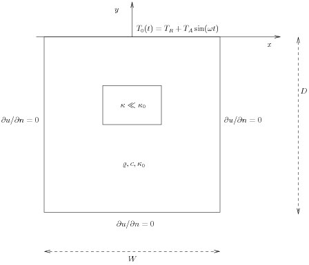
Sketch of a (2D) problem involving heating and cooling of the ground due to an oscillating surface temperature
The initial-boundary value problem for this problem reads
Here, \(\varrho\) is the density of the soil, \(c\) is the heat capacity, \(\kappa\) is the thermal conductivity (heat conduction coefficient) in the soil, and \(\Gamma_0\) is the surface boundary \(x_{d-1}=0\).
We use a \(\theta\)-scheme in time, i.e., the evolution equation \(\partial P/\partial t=Q(t)\) is discretized as
where \(\theta\in[0,1]\) is a weighting factor: \(\theta =1\) corresponds to the backward difference scheme, \(\theta =1/2\) to the Crank-Nicolson scheme, and \(\theta =0\) to a forward difference scheme. The \(\theta\)-scheme applied to our PDE results in
Bringing this time-discrete PDE into weak form follows the technique shown many times earlier in this tutorial. In the standard notation \(a(T,v)=L(v)\) the weak form has
Observe that boundary integrals vanish because of the Neumann boundary conditions.
The size of a 3D box is taken as \(W\times W\times D\), where \(D\) is the depth and \(W=D/2\) is the width. We give the degree of the basis functions at the command line, then \(D\), and then the divisions of the domain in the various directions. To make a box, rectangle, or interval of arbitrary (not unit) size, we have the DOLFIN classes BoxMesh, RectangleMesh, and IntervalMesh at our disposal. The mesh and the function space can be created by the following code:
degree = int(sys.argv[1])
D = float(sys.argv[2])
W = D/2.0
divisions = [int(arg) for arg in sys.argv[3:]]
d = len(divisions)  # no of space dimensions
if d == 1:
    mesh = IntervalMesh(divisions[0], -D, 0)
elif d == 2:
    mesh = RectangleMesh(-W/2, -D, W/2, 0, divisions[0], divisions[1])
elif d == 3:
    mesh = BoxMesh(-W/2, -W/2, -D, W/2, W/2, 0,
               divisions[0], divisions[1], divisions[2])
V = FunctionSpace(mesh, 'Lagrange', degree)
The RectangleMesh and BoxMesh objects are defined by the coordinates of the “minimum” and “maximum” corners.
Setting Dirichlet conditions at the upper boundary can be done by
T_R = 0; T_A = 1.0; omega = 2*pi

T_0 = Expression('T_R + T_A*sin(omega*t)',
                 T_R=T_R, T_A=T_A, omega=omega, t=0.0)

def surface(x, on_boundary):
    return on_boundary and abs(x[d-1]) < 1E-14

bc = DirichletBC(V, T_0, surface)
The \(\kappa\) function can be defined as a constant \(\kappa_1\) inside the particular rectangular area with a special soil composition, as indicated in Figure Sketch of a (2D) problem involving heating and cooling of the ground due to an oscillating surface temperature. Outside this area \(\kappa\) is a constant \(\kappa_0\). The domain of the rectangular area is taken as
in 3D, with \([-W/4, W/4]\times [-D/2, -D/2 + D/4]\) in 2D and \([-D/2, -D/2 + D/4]\) in 1D. Since we need some testing in the definition of the \(\kappa(\boldsymbol{x})\) function, the most straightforward approach is to define a subclass of Expression, where we can use a full Python method instead of just a C++ string formula for specifying a function. The method that defines the function is called eval:
class Kappa(Expression):
    def eval(self, value, x):
        """x: spatial point, value[0]: function value."""
        d = len(x)  # no of space dimensions
        material = 0  # 0: outside, 1: inside
        if d == 1:
            if -D/2. < x[d-1] < -D/2. + D/4.:
                material = 1
        elif d == 2:
            if -D/2. < x[d-1] < -D/2. + D/4. and \
               -W/4. < x[0] < W/4.:
                material = 1
        elif d == 3:
            if -D/2. < x[d-1] < -D/2. + D/4. and \
               -W/4. < x[0] < W/4. and -W/4. < x[1] < W/4.:
                material = 1
        value[0] = kappa_0 if material == 0 else kappa_1
The eval method gives great flexibility in defining functions, but a downside is that C++ calls up eval in Python for each point x, which is a slow process, and the number of calls is proportional to the number of nodes in the mesh. Function expressions in terms of strings are compiled to efficient C++ functions, being called from C++, so we should try to express functions as string expressions if possible. (The eval method can also be defined through C++ code, but this is much more complicated and not covered here.) Using inline if-tests in C++, we can make string expressions for \(\kappa\):
kappa_str = {}
kappa_str[1] = 'x[0] > -D/2 && x[0] < -D/2 + D/4 ? kappa_1 : kappa_0'
kappa_str[2] = 'x[0] > -W/4 && x[0] < W/4 '\
               '&& x[1] > -D/2 && x[1] < -D/2 + D/4 ? '\
               'kappa_1 : kappa_0'
kappa_str[3] = 'x[0] > -W/4 && x[0] < W/4 '\
               'x[1] > -W/4 && x[1] < W/4 '\
               '&& x[2] > -D/2 && x[2] < -D/2 + D/4 ?'\
               'kappa_1 : kappa_0'

kappa = Expression(kappa_str[d],
                   D=D, W=W, kappa_0=kappa_0, kappa_1=kappa_1)
Let T denote the unknown spatial temperature function at the current time level, and let T_1 be the corresponding function at one earlier time level. We are now ready to define the initial condition and the a and L forms of our problem:
T_prev = interpolate(Constant(T_R), V)

rho = 1
c = 1
period = 2*pi/omega
t_stop = 5*period
dt = period/20  # 20 time steps per period
theta = 1

T = TrialFunction(V)
v = TestFunction(V)
f = Constant(0)
a = rho*c*T*v*dx + theta*dt*kappa*\
    inner(nabla_grad(T), nabla_grad(v))*dx
L = (rho*c*T_prev*v + dt*f*v -
     (1-theta)*dt*kappa*inner(nabla_grad(T_1), nabla_grad(v)))*dx

A = assemble(a)
b = None  # variable used for memory savings in assemble calls
T = Function(V)   # unknown at the current time level
We could, alternatively, break a and L up in subexpressions and assemble a mass matrix and stiffness matrix, as exemplified in the section Avoiding Assembly, to avoid assembly of b at every time level. This modification is straightforward and left as an exercise. The speed-up can be significant in 3D problems.
The time loop is very similar to what we have displayed in the section Implementation (2):
T = Function(V)   # unknown at the current time level
t = dt
while t <= t_stop:
    b = assemble(L, tensor=b)
    T_0.t = t
    bc.apply(A, b)
    solve(A, T.vector(), b)
    # visualization statements
    t += dt
    T_prev.assign(T)
The complete code in sin_daD.py contains several statements related to visualization and animation of the solution, both as a finite element field (plot calls) and as a curve in the vertical direction. The code also plots the exact analytical solution,
which is valid when \(\kappa = \kappa_0=\kappa_1\).
Implementing this analytical solution as a Python function taking scalars and numpy arrays as arguments requires a word of caution. A straightforward function like
def T_exact(x):
    a = sqrt(omega*rho*c/(2*kappa_0))
    return T_R + T_A*exp(a*x)*sin(omega*t + a*x)
will not work and result in an error message from UFL. The reason is that the names exp and sin are those imported by the from dolfin import * statement, and these names come from UFL and are aimed at being used in variational forms. In the T_exact function where x may be a scalar or a numpy array, we therefore need to explicitly specify numpy.exp and numpy.sin:
def T_exact(x):
    a = sqrt(omega*rho*c/(2*kappa_0))
    return T_R + T_A*numpy.exp(a*x)*numpy.sin(omega*t + a*x)
The complete code is found in the file The reader is encouraged to play around with the code and test out various parameter sets:
- \(T_R=0\), \(T_A=1\), \(\kappa_0 = \kappa_1=0.2\), \(\varrho = c = 1\), \(\omega = 2\pi\)
- \(T_R=0\), \(T_A=1\), \(\kappa_0=0.2\), \(\kappa_1=0.01\), \(\varrho = c = 1\), \(\omega = 2\pi\)
- \(T_R=0\), \(T_A=1\), \(\kappa_0=0.2\), \(\kappa_1=0.001\), \(\varrho = c = 1\), \(\omega = 2\pi\)
- \(T_R=10\) C, \(T_A=10\) C, \(\kappa_0= 2.3 \hbox{ K}^{-1}\hbox{Ns}^{-1}\), \(\kappa_1= 100 \hbox{ K}^{-1}\hbox{Ns}^{-1}\), \(\varrho = 1500\hbox{ kg/m}^3\), \(c = 1480\hbox{ Nm}\cdot\hbox{kg}^{-1}\hbox{K}^{-1}\), \(\omega = 2\pi/24\) 1/h \(= 7.27\cdot 10^{-5}\) 1/s, \(D=1.5\) m
- As above, but \(\kappa_0= 12.3 \hbox{ K}^{-1}\hbox{Ns}^{-1}\) and \(\kappa_1= 10^4 \hbox{ K}^{-1}\hbox{Ns}^{-1}\)
Data set number 4 is relevant for real temperature variations in the ground (not necessarily the large value of \(\kappa_1\)), while data set number 5 exaggerates the effect of a large heat conduction contrast so that it becomes clearly visible in an animation.
Up to now we have been very fond of the unit square as domain, which is an appropriate choice for initial versions of a PDE solver. The strength of the finite element method, however, is its ease of handling domains with complex shapes. This section shows some methods that can be used to create different types of domains and meshes.
Domains of complex shape must normally be constructed in separate preprocessor programs. Two relevant preprocessors are Triangle for 2D domains and NETGEN for 3D domains.
DOLFIN has a few tools for creating various types of meshes over domains with simple shape: UnitIntervalMesh, UnitSquareMesh, UnitCubeMesh, IntervalMesh, RectangleMesh, BoxMesh, UnitCircleMesh, and UnitSphere.
Some of these names have been briefly met in previous sections. The hopefully self-explanatory code snippet below summarizes typical constructions of meshes with the aid of these tools:
# 1D domains
mesh = UnitIntervalMesh(20)     # 20 cells, 21 vertices
mesh = IntervalMesh(20, -1, 1)  # domain [-1,1]

# 2D domains (6x10 divisions, 120 cells, 77 vertices)
mesh = UnitSquareMesh(6, 10)  # 'right' diagonal is default
# The diagonals can be right, left or crossed
mesh = UnitSquareMesh(6, 10, 'left')
mesh = UnitSquareMesh(6, 10, 'crossed')

# Domain [0,3]x[0,2] with 6x10 divisions and left diagonals
mesh = RectangleMesh(0, 0, 3, 2, 6, 10, 'left')

# 6x10x5 boxes in the unit cube, each box gets 6 tetrahedra:
mesh = UnitCubeMesh(6, 10, 5)

# Domain [-1,1]x[-1,0]x[-1,2] with 6x10x5 divisions
mesh = BoxMesh(-1, -1, -1, 1, 0, 2, 6, 10, 5)

# 10 divisions in radial directions
mesh = UnitCircleMesh(10)
mesh = UnitSphere(10)
A mesh that is denser toward a boundary is often desired to increase accuracy in that region. Given a mesh with uniformly spaced coordinates \(x_0,\ldots,x_{M-1}\) in \([a,b]\), the coordinate transformation \(\xi = (x-a)/(b-a)\) maps \(x\) onto \(\xi\in [0,1]\). A new mapping \(\eta = \xi^s\), for some \(s>1\), stretches the mesh toward \(\xi=0\) (\(x=a\)), while \(\eta = \xi^{1/s}\) makes a stretching toward \(\xi=1\) (\(x=b\)). Mapping the \(\eta\in[0,1]\) coordinates back to \([a,b]\) gives new, stretched \(x\) coordinates,
toward \(x=a\), or
toward \(x=b\)
One way of creating more complex geometries is to transform the vertex coordinates in a rectangular mesh according to some formula. Say we want to create a part of a hollow cylinder of \(\Theta\) degrees, with inner radius \(a\) and outer radius \(b\). A standard mapping from polar coordinates to Cartesian coordinates can be used to generate the hollow cylinder. Given a rectangle in \((\bar x, \bar y)\) space such that \(a\leq \bar x\leq b\) and \(0\leq \bar y\leq 1\), the mapping
takes a point in the rectangular \((\bar x,\bar y)\) geometry and maps it to a point \((\hat x, \hat y)\) in a hollow cylinder.
The corresponding Python code for first stretching the mesh and then mapping it onto a hollow cylinder looks as follows:
Theta = pi/2
a, b = 1, 5.0
nr = 10  # divisions in r direction
nt = 20  # divisions in theta direction
mesh = RectangleMesh(a, 0, b, 1, nr, nt, 'crossed')

# First make a denser mesh towards r=a
x = mesh.coordinates()[:,0]
y = mesh.coordinates()[:,1]
s = 1.3

def denser(x, y):
    return [a + (b-a)*((x-a)/(b-a))**s, y]

x_bar, y_bar = denser(x, y)
xy_bar_coor = numpy.array([x_bar, y_bar]).transpose()
mesh.coordinates()[:] = xy_bar_coor
plot(mesh, title='stretched mesh')

def cylinder(r, s):
    return [r*numpy.cos(Theta*s), r*numpy.sin(Theta*s)]

x_hat, y_hat = cylinder(x_bar, y_bar)
xy_hat_coor = numpy.array([x_hat, y_hat]).transpose()
mesh.coordinates()[:] = xy_hat_coor
plot(mesh, title='hollow cylinder')
interactive()
The result of calling denser and cylinder above is a list of two vectors, with the \(x\) and \(y\) coordinates, respectively. Turning this list into a numpy array object results in a \(2\times M\) array, \(M\) being the number of vertices in the mesh. However, mesh.coordinates() is by a convention an \(M\times 2\) array so we need to take the transpose. The resulting mesh is displayed in Figure Hollow cylinder generated by mapping a rectangular mesh, stretched toward the left side.
Hollow cylinder generated by mapping a rectangular mesh, stretched toward the left side
Setting boundary conditions in meshes created from mappings like the one illustrated above is most conveniently done by using a mesh function to mark parts of the boundary. The marking is easiest to perform before the mesh is mapped since one can then conceptually work with the sides in a pure rectangle.
Solving PDEs in domains made up of different materials is a frequently encountered task. In FEniCS, these kind of problems are handled by defining subdomains inside the domain. The subdomains may represent the various materials. We can thereafter define material properties through functions, known in FEniCS as mesh functions, that are piecewise constant in each subdomain. A simple example with two materials (subdomains) in 2D will demonstrate the basic steps in the process.
Suppose we want to solve
in a domain \(\Omega\) consisting of two subdomains where \(k\) takes on a different value in each subdomain. For simplicity, yet without loss of generality, we choose for the current implementation the domain \(\Omega = [0,1]\times [0,1]\) and divide it into two equal subdomains,
We define \(k(x,y)=k_0\) in \(\Omega_0\) and \(k(x,y)=k_1\) in \(\Omega_1\), where \(k_0>0\) and \(k_1>0\) are given constants. As boundary conditions, we choose \(u=0\) at \(y=0\), \(u=1\) at \(y=1\), and \(\partial u/\partial n=0\) at \(x=0\) and \(x=1\). One can show that the exact solution is now given by
As long as the element boundaries coincide with the internal boundary \(y=1/2\), this piecewise linear solution should be exactly recovered by Lagrange elements of any degree. We use this property to verify the implementation.
Physically, the present problem may correspond to heat conduction, where the heat conduction in \(\Omega_1\) is ten times more efficient than in \(\Omega_0\). An alternative interpretation is flow in porous media with two geological layers, where the layers’ ability to transport the fluid differs by a factor of 10.
The new functionality in this subsection regards how to define the subdomains \(\Omega_0\) and \(\Omega_1\). For this purpose we need to use subclasses of class SubDomain, not only plain functions as we have used so far for specifying boundaries. Consider the boundary function
def boundary(x, on_boundary):
    tol = 1E-14
    return on_boundary and abs(x[0]) < tol
for defining the boundary \(x=0\). Instead of using such a stand-alone function, we can create an instance (or object) of a subclass of SubDomain, which implements the inside method as an alternative to the boundary function:
class Boundary(SubDomain):
    def inside(self, x, on_boundary):
        tol = 1E-14
        return on_boundary and abs(x[0]) < tol

boundary = Boundary()
bc = DirichletBC(V, Constant(0), boundary)
A word about computer science terminology may be used here: The term instance means a Python object of a particular type (such as SubDomain, Function FunctionSpace, etc.). Many use instance and object as interchangeable terms. In other computer programming languages one may also use the term variable for the same thing. We mostly use the well-known term object in this text.
A subclass of SubDomain with an inside method offers functionality for marking parts of the domain or the boundary. Now we need to define one class for the subdomain \(\Omega_0\) where \(y\leq 1/2\) and another for the subdomain \(\Omega_1\) where \(y\geq 1/2\):
class Omega0(SubDomain):
    def inside(self, x, on_boundary):
        return True if x[1] <= 0.5 else False

class Omega1(SubDomain):
    def inside(self, x, on_boundary):
        return True if x[1] >= 0.5 else False
Notice the use of <= and >= in both tests. For a cell to belong to, e.g., \(\Omega_1\), the inside method must return True for all the vertices x of the cell. So to make the cells at the internal boundary \(y=1/2\) belong to \(\Omega_1\), we need the test x[1] >= 0.5.
The next task is to use a MeshFunction to mark all cells in \(\Omega_0\) with the subdomain number 0 and all cells in \(\Omega_1\) with the subdomain number 1. Our convention is to number subdomains as \(0,1,2,\ldots\).
A MeshFunction is a discrete function that can be evaluated at a set of so-called mesh entities. Examples of mesh entities are cells, facets, and vertices. A MeshFunction over cells is suitable to represent subdomains (materials), while a MeshFunction over facets is used to represent pieces of external or internal boundaries. Mesh functions over vertices can be used to describe continuous fields.
Since we need to define subdomains of \(\Omega\) in the present example, we must make use of a MeshFunction over cells. The MeshFunction constructor is fed with three arguments: 1) the type of value: 'int' for integers, 'uint' for positive (unsigned) integers, 'double' for real numbers, and 'bool' for logical values; 2) a Mesh object, and 3) the topological dimension of the mesh entity in question: cells have topological dimension equal to the number of space dimensions in the PDE problem, and facets have one dimension lower. Alternatively, the constructor can take just a filename and initialize the MeshFunction from data in a file.
We start with creating a MeshFunction whose values are non-negative integers ('uint') for numbering the subdomains. The mesh entities of interest are the cells, which have dimension 2 in a two-dimensional problem (1 in 1D, 3 in 3D). The appropriate code for defining the MeshFunction for two subdomains then reads
subdomains = MeshFunction('uint', mesh, 2)
# Mark subdomains with numbers 0 and 1
subdomain0 = Omega0()
subdomain0.mark(subdomains, 0)
subdomain1 = Omega1()
subdomain1.mark(subdomains, 1)
Calling subdomains.array() returns a numpy array of the subdomain values. That is, subdomain.array()[i] is the subdomain value of cell number i. This array is used to look up the subdomain or material number of a specific element.
We need a function k that is constant in each subdomain \(\Omega_0\) and \(\Omega_1\). Since we want k to be a finite element function, it is natural to choose a space of functions that are constant over each element. The family of discontinuous Galerkin methods, in FEniCS denoted by 'DG', is suitable for this purpose. Since we want functions that are piecewise constant, the value of the degree parameter is zero:
V0 = FunctionSpace(mesh, 'DG', 0)
k  = Function(V0)
To fill k with the right values in each element, we loop over all cells (i.e., indices in subdomain.array()), extract the corresponding subdomain number of a cell, and assign the corresponding \(k\) value to the k.vector() array:
k_values = [1.5, 50]  # values of k in the two subdomains
for cell_no in range(len(subdomains.array())):
    subdomain_no = subdomains.array()[cell_no]
    k.vector()[cell_no] = k_values[subdomain_no]
Long loops in Python are known to be slow, so for large meshes it is preferable to avoid such loops and instead use vectorized code. Normally this implies that the loop must be replaced by calls to functions from the numpy library that operate on complete arrays (in efficient C code). The functionality we want in the present case is to compute an array of the same size as subdomain.array(), but where the value i of an entry in subdomain.array() is replaced by k_values[i]. Such an operation is carried out by the numpy function choose:
help = numpy.asarray(subdomains.array(), dtype=numpy.int32)
k.vector()[:] = numpy.choose(help, k_values)
The help array is required since choose cannot work with subdomain.array() because this array has elements of type uint32. We must therefore transform this array to an array help with standard int32 integers.
Having the k function ready for finite element computations, we can proceed in the normal manner with defining essential boundary conditions, as in the section Multiple Dirichlet Conditions, and the \(a(u,v)\) and \(L(v)\) forms, as in the section A Variable-Coefficient Poisson Problem. All the details can be found in the file mat2_p2D.py.
Let us go back to the model problem from the section Multiple Dirichlet Conditions where we had both Dirichlet and Neumann conditions. The term v*g*ds in the expression for L implies a boundary integral over the complete boundary, or in FEniCS terms, an integral over all exterior facets. However, the contributions from the parts of the boundary where we have Dirichlet conditions are erased when the linear system is modified by the Dirichlet conditions. We would like, from an efficiency point of view, to integrate v*g*ds only over the parts of the boundary where we actually have Neumann conditions. And more importantly, in other problems one may have different Neumann conditions or other conditions like the Robin type condition. With the mesh function concept we can mark different parts of the boundary and integrate over specific parts. The same concept can also be used to treat multiple Dirichlet conditions. The forthcoming text illustrates how this is done.
Essentially, we still stick to the model problem from the section Multiple Dirichlet Conditions, but replace the Neumann condition at \(y=0\) by a Robin condition:
where \(p\) and \(q\) are specified functions. The Robin condition is most often used to model heat transfer to the surroundings and arise naturally from Newton’s cooling law.
Since we have prescribed a simple solution in our model problem, \(u=1+x^2+2y^2\), we adjust \(p\) and \(q\) such that the condition holds at \(y=0\). This implies that \(q=1+x^2+2y^2\) and \(p\) can be arbitrary (the normal derivative at \(y=0\): \(\partial u/\partial n = -\partial u/\partial y = -4y=0\)).
Now we have four parts of the boundary: \(\Gamma_N\) which corresponds to the upper side \(y=1\), \(\Gamma_R\) which corresponds to the lower part \(y=0\), \(\Gamma_0\) which corresponds to the left part \(x=0\), and \(\Gamma_1\) which corresponds to the right part \(x=1\). The complete boundary-value problem reads
The involved prescribed functions are \(u_L= 1 + 2y^2\), \(u_R = 2 + 2y^2\), \(q=1+x^2+2y^2\), \(p\) is arbitrary, and \(g=-4y\).
Integration by parts of \(-\int_\Omega v\nabla^2 u {\, \mathrm{d}x}\) becomes as usual
The boundary integral vanishes on \(\Gamma_0\cup\Gamma_1\), and we split the parts over \(\Gamma_N\) and \(\Gamma_R\) since we have different conditions at those parts:
The weak form then becomes
We want to write this weak form in the standard notation \(a(u,v)=L(v)\), which requires that we identify all integrals with both \(u\) and \(v\), and collect these in \(a(u,v)\), while the remaining integrals with \(v\) and not \(u\) go into \(L(v)\). The integral from the Robin condition must of this reason be split in two parts:
We then have
A natural starting point for implementation is the dn2_p2D.py program in the directory stationary/poisson. The new aspects are
- definition of a mesh function over the boundary,
- marking each side as a subdomain, using the mesh function,
- splitting a boundary integral into parts.
Task 1 makes use of the MeshFunction object, but contrary to the section Implementation (3), this is not a function over cells, but a function over cell facets. The topological dimension of cell facets is one lower than the cell interiors, so in a two-dimensional problem the dimension becomes 1. In general, the facet dimension is given as mesh.topology().dim()-1, which we use in the code for ease of direct reuse in other problems. The construction of a MeshFunction object to mark boundary parts now reads
boundary_parts = \
  MeshFunction("uint", mesh, mesh.topology().dim()-1)
As in the section Implementation (3) we use a subclass of SubDomain to identify the various parts of the mesh function. Problems with domains of more complicated geometries may set the mesh function for marking boundaries as part of the mesh generation. In our case, the \(y=0\) boundary can be marked by
class LowerRobinBoundary(SubDomain):
    def inside(self, x, on_boundary):
        tol = 1E-14   # tolerance for coordinate comparisons
        return on_boundary and abs(x[1]) < tol

Gamma_R = LowerRobinBoundary()
Gamma_R.mark(boundary_parts, 0)
The code for the \(y=1\) boundary is similar and is seen in dnr_p2D.py.
The Dirichlet boundaries are marked similarly, using subdomain number 2 for \(\Gamma_0\) and 3 for \(\Gamma_1\):
class LeftBoundary(SubDomain):
    def inside(self, x, on_boundary):
        tol = 1E-14   # tolerance for coordinate comparisons
        return on_boundary and abs(x[0]) < tol

Gamma_0 = LeftBoundary()
Gamma_0.mark(boundary_parts, 2)

class RightBoundary(SubDomain):
    def inside(self, x, on_boundary):
        tol = 1E-14   # tolerance for coordinate comparisons
        return on_boundary and abs(x[0] - 1) < tol

Gamma_1 = RightBoundary()
Gamma_1.mark(boundary_parts, 3)
Specifying the DirichletBC objects may now make use of the mesh function (instead of a SubDomain subclass object) and an indicator for which subdomain each condition should be applied to:
u_L = Expression('1 + 2*x[1]*x[1]')
u_R = Expression('2 + 2*x[1]*x[1]')
bcs = [DirichletBC(V, u_L, boundary_parts, 2),
       DirichletBC(V, u_R, boundary_parts, 3)]
Some functions need to be defined before we can go on with the a and L of the variational problem:
g = Expression('-4*x[1]')
q = Expression('1 + x[0]*x[0] + 2*x[1]*x[1]')
p = Constant(100)  # arbitrary function can go here
u = TrialFunction(V)
v = TestFunction(V)
f = Constant(-6.0)
The new aspect of the variational problem is the two distinct boundary integrals. Having a mesh function over exterior cell facets (our boundary_parts object), where subdomains (boundary parts) are numbered as \(0,1,2,\ldots\), the special symbol ds(0) implies integration over subdomain (part) 0, ds(1) denotes integration over subdomain (part) 1, and so on. The idea of multiple ds-type objects generalizes to volume integrals too: dx(0), dx(1), etc., are used to integrate over subdomain 0, 1, etc., inside \(\Omega\).
The variational problem can be defined as
a = inner(nabla_grad(u), nabla_grad(v))*dx + p*u*v*ds(0)
L = f*v*dx - g*v*ds(1) + p*q*v*ds(0)
For the ds(0) and ds(1) symbols to work we must obviously connect them (or a and L) to the mesh function marking parts of the boundary. This is done by a certain keyword argument to the assemble function:
A = assemble(a, exterior_facet_domains=boundary_parts)
b = assemble(L, exterior_facet_domains=boundary_parts)
Then essential boundary conditions are enforced, and the system can be solved in the usual way:
for bc in bcs:
    bc.apply(A, b)
u = Function(V)
U = u.vector()
solve(A, U, b)
The complete code is in the dnr_p2D.py file in the stationary/poisson directory.
Many more topics could be treated in a FEniCS tutorial, e.g., how to solve systems of PDEs, how to work with mixed finite element methods, how to create more complicated meshes and mark boundaries, and how to create more advanced visualizations. However, to limit the size of this tutorial, the examples end here. There are, fortunately, a rich set of FEniCS demos. The FEniCS documentation explains a collection of PDE solvers in detail: the Poisson equation, the mixed formulation for the Poission equation, the Biharmonic equation, the equations of hyperelasticity, the Cahn-Hilliard equation, and the incompressible Navier-Stokes equations. Both Python and C++ versions of these solvers are explained. An eigenvalue solver is also documented. In the dolfin/demo directory of the DOLFIN source code tree you can find programs for these and many other examples, including the advection-diffusion equation, the equations of elastodynamics, a reaction-diffusion equation, various finite element methods for the Stokes problem, discontinuous Galerkin methods for the Poisson and advection-diffusion equations, and an eigenvalue problem arising from electromagnetic waveguide problem with Nedelec elements. There are also numerous demos on how to apply various functionality in FEniCS, e.g., mesh refinement and error control, moving meshes (for ALE methods), computing functionals over subsets of the mesh (such as lift and drag on bodies in flow), and creating separate subdomain meshes from a parent mesh.
The project cbc.solve (https://launchpad.net/cbc.solve) offers more complete PDE solvers for the Navier-Stokes equations, the equations of hyperelasticity, fluid-structure interaction, viscous mantle flow, and the bidomain model of electrophysiology. Most of these solvers are described in the “FEniCS book” [Ref01] (https://launchpad.net/fenics-book). Another project, cbc.rans (https://launchpad.net/cbc.rans), offers an environment for very flexible and easy implementation of Navier-Stokes solvers and turbulence [Ref02] [Ref03]. For example, cbc.rans contains an elliptic relaxation model for turbulent flow involving 18 nonlinear PDEs. FEniCS proved to be an ideal environment for implementing such complicated PDE models. The easy construction of systems of nonlinear PDEs in cbc.rans has been further generalized to simplify the implementation of large systems of nonlinear PDEs in general. The functionality is found in the cbc.pdesys package (https://launchpad.net/cbcpdesys).
Below we explain some key terms used in this tutorial.
- FEniCS: name of a software suite composed of many individual software
- components (see fenicsproject.org). Some components are DOLFIN and Viper, explicitly referred to in this tutorial. Others are FFC and FIAT, heavily used by the programs appearing in this tutorial, but never explicitly used from the programs.
- DOLFIN: a FEniCS component, more precisely a C++ library, with
- a Python interface, for performing important actions in finite element programs. DOLFIN makes use of many other FEniCS components and many external software packages.
- Viper: a FEniCS component for quick visualization of finite element
- meshes and solutions.
- UFL: a FEniCS component implementing the unified form language
- for specifying finite element forms in FEniCS programs. The definition of the forms, typically called a and L in this tutorial, must have legal UFL syntax. The same applies to the definition of functionals (see the section Computing Functionals).
- Class (Python): a programming construction for creating objects
- containing a set of variables and functions. Most types of FEniCS objects are defined through the class concept.
- Instance (Python): an object of a particular type, where the type is
- implemented as a class. For instance, mesh = UnitIntervalMesh(10) creates an instance of class UnitIntervalMesh, which is reached by the name mesh. (Class UnitIntervalMesh is actually just an interface to a corresponding C++ class in the DOLFIN C++ library.)
- Class method (Python): a function in a class, reached by dot
- notation: instance_name.method_name
- argument self (Python): required first parameter in class methods,
- representing a particular object of the class. Used in method definitions, but never in calls to a method. For example, if method(self, x) is the definition of method in a class Y, method is called as y.method(x), where y is an instance of class Y. In a call like y.method(x), method is invoked with self=y.
- Class attribute (Python): a variable in a class, reached by
- dot notation: instance_name.attribute_name
Most classes in FEniCS have an explanation of the purpose and usage that can be seen by using the general documentation command pydoc for Python objects. You can type
pydoc dolfin.X
to look up documentation of a Python class X from the DOLFIN library (X can be UnitSquareMesh, Function, Viper, etc.). Below is an overview of the most important classes and functions in FEniCS programs, in the order they typically appear within programs.
UnitSquareMesh(nx, ny): generate mesh over the unit square \([0,1]\times [0,1]\) using nx divisions in \(x\) direction and ny divisions in \(y\) direction. Each of the nx*ny squares are divided into two cells of triangular shape.
UnitIntervalMesh, UnitCubeMesh, UnitCircleMesh, UnitSphere, IntervalMesh, RectangleMesh, and BoxMesh: generate mesh over domains of simple geometric shape, see the section Creating More Complex Domains.
FunctionSpace(mesh, element_type, degree): a function space defined over a mesh, with a given element type (e.g., 'Lagrange' or 'DG'), with basis functions as polynomials of a specified degree.
Expression(formula, p1=v1, p2=v2, ...): a scalar- or vector-valued function, given as a mathematical expression formula (string) written in C++ syntax. The spatial coordinates in the expression are named x[0], x[1], and x[2], while time and other physical parameters can be represented as symbols p1, p2, etc., with corresponding values v1, v2, etc., initialized through keyword arguments. These parameters become attributes, whose values can be modified when desired.
Function(V): a scalar- or vector-valued finite element field in the function space V. If V is a FunctionSpace object, Function(V) becomes a scalar field, and with V as a VectorFunctionSpace object, Function(V) becomes a vector field.
SubDomain: class for defining a subdomain, either a part of the boundary, an internal boundary, or a part of the domain. The programmer must subclass SubDomain and implement the inside(self, x, on_boundary) function (see the section Implementation (1)) for telling whether a point x is inside the subdomain or not.
Mesh: class for representing a finite element mesh, consisting of cells, vertices, and optionally faces, edges, and facets.
MeshFunction: tool for marking parts of the domain or the boundary. Used for variable coefficients (“material properties”, see the section Working with Two Subdomains) or for boundary conditions (see the section Multiple Neumann, Robin, and Dirichlet Condition).
DirichletBC(V, value, where): specification of Dirichlet (essential) boundary conditions via a function space V, a function value(x) for computing the value of the condition at a point x, and a specification where of the boundary, either as a SubDomain subclass instance, a plain function, or as a MeshFunction instance. In the latter case, a 4th argument is provided to describe which subdomain number that describes the relevant boundary.
TestFunction(V): define a test function on a space V to be used in a variational form.
TrialFunction(V): define a trial function on a space V to be used in a variational form to represent the unknown in a finite element problem.
assemble(X): assemble a matrix, a right-hand side, or a functional, given a from X written with UFL syntax.
assemble_system(a, L, bcs): assemble the matrix and the right-hand side from a bilinear (a) and linear (L) form written with UFL syntax. The bcs parameter holds one or more DirichletBC objects.
LinearVariationalProblem(a, L, u, bcs): define a variational problem, given a bilinear (a) and linear (L) form, written with UFL syntax, and one or more DirichletBC objects stored in bcs.
LinearVariationalSolver(problem): create solver object for a linear variational problem object (problem).
solve(A, U, b): solve a linear system with A as coefficient matrix (Matrix object), U as unknown (Vector object), and b as right-hand side (Vector object). Usually, U = u.vector(), where u is a Function object representing the unknown finite element function of the problem, while A and b are computed by calls to assemble or assemble_system.
plot(q): quick visualization of a mesh, function, or mesh function q, using the Viper component in FEniCS.
interpolate(func, V): interpolate a formula or finite element function func onto the function space V.
project(func, V): project a formula or finite element function func onto the function space V.
When defining a function in terms of a mathematical expression inside a string formula, e.g.,
myfunc = Expression('sin(x[0])*cos(x[1])')
the expression contained in the first argument will be turned into a C++ function and compiled to gain efficiency. Therefore, the syntax used in the expression must be valid C++ syntax. Most Python syntax for mathematical expressions are also valid C++ syntax, but power expressions make an exception: p**a must be written as pow(p,a) in C++ (this is also an alternative Python syntax). The following mathematical functions can be used directly in C++ expressions when defining Expression objects: cos, sin, tan, acos, asin, atan, atan2, cosh, sinh, tanh, exp, frexp, ldexp, log, log10, modf, pow, sqrt, ceil, fabs, floor, and fmod. Moreover, the number \(\pi\) is available as the symbol pi. All the listed functions are taken from the cmath C++ header file, and one may hence consult documentation of cmath for more information on the various functions.
Parameters in expression strings must be initialized via keyword arguments when creating the Expression object:
myfunc = Expression('sin(w_x*x[0])*cos(w_y*x[1])',
                     w_x=pi, w_y=2*pi)
The following solution methods for linear systems can be accessed in FEniCS programs:
| Name | Method |
|---|---|
| 'lu' | sparse LU factorization (Gaussian elim.) |
| 'cholesky' | sparse Cholesky factorization |
| 'cg' | Conjugate gradient method |
| 'gmres' | Generalized minimal residual method |
| 'bicgstab' | Biconjugate gradient stabilized method |
| 'minres' | Minimal residual method |
| 'tfqmr' | Transpose-free quasi-minimal residual method |
| 'richardson' | Richardson method |
Possible choices of preconditioners include
| Name | Method |
|---|---|
| 'none' | No preconditioner |
| 'ilu' | Incomplete LU factorization |
| 'icc' | Incomplete Cholesky factorization |
| 'jacobi' | Jacobi iteration |
| 'bjacobi' | Block Jacobi iteration |
| 'sor' | Successive over-relaxation |
| 'amg' | Algebraic multigrid (BoomerAMG or ML) |
| 'additive_schwarz' | Additive Schwarz |
| 'hypre_amg' | Hypre algebraic multigrid (BoomerAMG) |
| 'hypre_euclid' | Hypre parallel incomplete LU factorization |
| 'hypre_parasails' | Hypre parallel sparse approximate inverse |
| 'ml_amg' | ML algebraic multigrid |
Many of the choices listed above are only offered by a specific backend, so setting the backend appropriately is necessary for being able to choose a desired linear solver or preconditioner.
An up-to-date list of the available solvers and preconditioners in FEniCS can be produced by
list_linear_solver_methods()
list_krylov_solver_preconditioners()
The linear algebra backend determines the specific data structures that are used in the Matrix and Vector classes. For example, with the PETSc backend, Matrix encapsulates a PETSc matrix storage structure, and Vector encapsulates a PETSc vector storage structure. Sometimes one wants to perform operations directly on (say) the underlying PETSc objects. These can be fetched by
A_PETSc =
down_cast(A).mat() b_PETSc = down_cast(b).vec() U_PETSc =
down_cast(u.vector()).vec()
Here, u is a Function, A is a Matrix, and b is a Vector. The same syntax applies if we want to fetch the underlying Epetra, uBLAS, or MTL4 matrices and vectors.
Sometimes one wants to implement tailored solution algorithms, using special features of the underlying numerical packages. Here is an example where we create an ML preconditioned Conjugate Gradient solver by programming with Trilinos-specific objects directly. Given a linear system \(AU=b\), represented by a Matrix object A, and two Vector objects U and b in a Python program, the purpose is to set up a solver using the Aztec Conjugate Gradient method from Trilinos’ Aztec library and combine that solver with the algebraic multigrid preconditioner ML from the ML library in Trilinos. Since the various parts of Trilinos are mirrored in Python through the PyTrilinos package, we can operate directly on Trilinos-specific objects.
try:
    from PyTrilinos import Epetra, AztecOO, TriUtils, ML
except:
    print '''You Need to have PyTrilinos with
Epetra, AztecOO, TriUtils and ML installed
for this demo to run'''
    exit()

from dolfin import *

if not has_la_backend('Epetra'):
    print 'Warning: Dolfin is not compiled with Trilinos'
    exit()

parameters['linear_algebra_backend'] = 'Epetra'

# create matrix A and vector b in the usual way
# u is a Function

# Fetch underlying Epetra objects
A_epetra = down_cast(A).mat()
b_epetra = down_cast(b).vec()
U_epetra = down_cast(u.vector()).vec()

# Sets up the parameters for ML using a python dictionary
ML_param = {"max levels"        : 3,
            "output"            : 10,
            "smoother: type"    : "ML symmetric Gauss-Seidel",
            "aggregation: type" : "Uncoupled",
            "ML validate parameter list" : False
}

# Create the preconditioner
prec = ML.MultiLevelPreconditioner(A_epetra, False)
prec.SetParameterList(ML_param)
prec.ComputePreconditioner()

# Create solver and solve system
solver = AztecOO.AztecOO(A_epetra, U_epetra, b_epetra)
solver.SetPrecOperator(prec)
solver.SetAztecOption(AztecOO.AZ_solver, AztecOO.AZ_cg)
solver.SetAztecOption(AztecOO.AZ_output, 16)
solver.Iterate(MaxIters=1550, Tolerance=1e-5)

plot(u)
The FEniCS software components are available for Linux, Windows and Mac OS X platforms. Detailed information on how to get FEniCS running on such machines are available at the fenicsproject.org website. Here are just some quick descriptions and recommendations by the author.
To make the installation of FEniCS as painless and reliable as possible, I strongly recommend to use Ubuntu Linux. (Even though Mac users now can get FEniCS by a one-click install, I recommend using Ubuntu on Mac, unless you have significant experience with compiling and linking C++ libraries on Mac OS X.) Any standard PC can easily be equipped with Ubuntu Linux, which may live side by side with either Windows or Mac OS X or another Linux installation.
On Windows you can use the tool Wubi to automatically install Ubuntu in a dual boot fashion. A very popular alternative is to run Ubuntu in a separate window in your existing operation system, using a virtual machine. There are several virtual machine solutions to chose among, e.g., the free VirtualBox or the commercial tool VMWare Fusion. VirtualBox works well for many, but there might be hardware integration problems on Mac, so the superior VMWare Fusion tool is often worth the investment. The author has a description of how to install Ubuntu in a VMWare Fusion virtual machine.
Once Ubuntu is up and running, FEniCS is painlessly installed by
sudo apt-get install fenics
Sometimes the FEniCS software in a standard Ubuntu installation lacks some recent features and bug fixes. Go to fenicsproject.org, click on Download and then the Ubuntu logo, move down to Ubuntu PPA and copy a few Unix commands ot install the newest version of the FEniCS software.
A different type of virtual machine technology is Vagrant, which allows you to download a big file with a complete Ubuntu environment and run that environment in a terminal window on your Mac or Windows computer. This Ubuntu machine is integrated with the file system on your computer. The author has made a Vagrant box with most of the scientific computing software you need for programming with FEniCS, see a preliminary guide for download, installation, and usage.
The FEniCS installation also features a set of demo programs. These are stored in locations depending on the type of operating system. For Ubuntu the programs are stored in /usr/share/dolfin/demo.
The graphical user interface (GUI) of Ubuntu is quite similar to both Windows and Mac OS X, but to be efficient when doing science with FEniCS I recommend to run programs in a terminal window and write them in a text editor like Emacs or Vim. You can employ an integrated development environment such as Eclipse, but intensive FEniCS developers and users tend to find terminal windows and plain text editors more efficient and user friendly.
There are a large number of books on the finite element method. The books typically fall in either of two categories: the abstract mathematical version of the method and the engineering “structural analysis” formulation. FEniCS builds heavily on concepts in the abstract mathematical exposition. An easy-to-read book, which provides a good general background for using FEniCS, is Gockenbach [Ref04]. The book by Donea and Huerta [Ref05] has a similar style, but aims at readers with interest in fluid flow problems. Hughes [Ref06] is also highly recommended, especially for those interested in solid mechanics and heat transfer applications.
Readers with background in the engineering “structural analysis” version of the finite element method may find Bickford [Ref07] as an attractive bridge over to the abstract mathematical formulation that FEniCS builds upon. Those who have a weak background in differential equations in general should consult a more fundamental book, and Eriksson {em et al}. [Ref08] is a very good choice. On the other hand, FEniCS users with a strong background in mathematics and interest in the mathematical properties of the finite element method, will appreciate the texts by Brenner and Scott [Ref09], Braess [Ref10], Ern and Guermond [Ref11], Quarteroni and Valli [Ref12], or Ciarlet [Ref13].
Two very popular introductory books on Python are “Learning Python” by Lutz [Ref14] and “Practical Python” by Hetland [Ref15]. More advanced and comprehensive books include “Programming Python” by Lutz [Ref16], and “Python Cookbook” [Ref17] and “Python in a Nutshell” [Ref18] by Martelli. The web page http://wiki.python.org/moin/PythonBooks lists numerous additional books. Very few texts teach Python in a mathematical and numerical context, but the references [Ref19] [Ref20] [Ref21] are exceptions.
The author is very thankful to Johan Hake, Anders Logg, Kent-Andre Mardal, and Kristian Valen-Sendstad for promptly answering all my questions about FEniCS functionality and for implementing all my requests. I will in particular thank Professor Douglas Arnold for very valuable feedback on the text. Øystein Sørensen pointed out a lot of typos and contributed with many helpful comments. Many errors and typos were also reported by Mauricio Angeles, Ida Drøsdal, Hans Ekkehard Plesser, and Marie Rognes. Ekkehard Ellmann as well as two anonymous reviewers provided a series of suggestions and improvements.
Expressions and variational forms in a FEniCS program need to be compiled to C++ and linked with libraries if the expressions or forms have been modified since last time they were compiled. The tool Instant, which is part of the FEniCS software suite, is used for compiling and linking C++ code so that it can be used with Python.
Sometimes the compilation fails. You can see from the series of error messages which statement in the Python program that led to a compilation problem. Make sure to scroll back and identify whether the problematic line is associated with an expression, variational form, or the solve step.
The final line in the output of error messages points to a log file from the compilation where one can examine the error messages from the compiler. It is usually the last lines of this log file that are of interest. Occasionally, the compiler’s message can quickly lead to an understanding of the problem. A more fruitful approach is normally to examine the below list of common compilation problems and their remedies.
Instant remembers information about previous compilations and versions of your program. Sometimes removal of this information can solve the problem. Just run
instant-clean
in a terminal window whenever you encounter a compilation problem.
If the compilation problem arises from line with an Expression object, examine the syntax of the expression carefully. The section User-Defined Functions contains some information on valid syntax. You may also want to examine the log file, pointed to in the last line in the output of error messages. The compiler’s message about the syntax problem may lead you to a solution.
Some common problems are
- using a**b for exponentiation (illegal in C++) instead of pow(a, b),
- forgetting that the spatial coordinates are denoted by a vector x,
- forgetting that the \(x\), \(y\), and \(z\) coordinates in space correspond to x[0], x[1], and x[2], respectively.
Failure to initialize parameters in the expressions lead to a compilation error where this problem is explicitly pointed out.
Sometimes the problem lies in the solve step where a variational form is turned into a system of algebraic equations. The error message Unable to extract all indicies points to a problem with the variational form. Common errors include
- missing either the TrialFunction or the TestFunction object,
- no terms without TrialFunction objects.
- mathematically invalid operations in the variational form.
The first problem implies that one cannot make a matrix system or system of nonlinear algebraic equations out of the variational form. The second problem means that there is no “right-hand side” terms in the PDE with known quantities. Sometimes this is seemingly the case mathematically because the “right-hand side” is zero. Variational forms must represent this case as Constant(0)*v*dx where v is a TestFunction object. An example of the third problem is to take the inner product of a scalar and a vector (causing in this particular case the error message to be “Shape mismatch”).
The message Unable to extract common cell; missing cell definition in form or expression will typically arise from a term in the form where a test function (holding mesh and cell information) is missing. For example, a zero right-hand side Constant(0)*dx will generate this error.
One common reason for the above error message is that a form is written without being multiplied by dx or ds.
One reason may be that there are mathematical functions like sin and exp operating on numpy arrays. The problem is that the from dolfin import * statement imports sin, cos, and similar mathematical functions from UFL and these are aimed at taking Function or ``TrialFunction` objects as arguments and not numpy arrays. The remedy is to use prefix mathematical functions aimed at numpy arrays with numpy, or np if numpy is imported as np: numpy.exp or np.exp, for instance. Normally, boundary conditions and analytical solutions are represented by Expression objects and then this problem does not arise. The problem usually arises when pure Python functions with, e.g., analytical solutions are introduced for, e.g., plotting.
When encoutering a compilation problem where the Instant log file says something about missing double quote in an Expression, try compiling a previously working program. If that program faces the same problem, reboot Ubuntu and try again. If the problem persists, try running the Update Manager (because unfinished updates can cause compiler problems), reboot and try again.
You have forgotten to insert emp{interactive()} as the last statement in the program.
Run the command instant-clean to ensure that everything is (re)compiled. Check the formulas in string expressions carefully, and make sure that divisions do not lead to integer division (i.e., at least one of the operands in a division must be a floating-point variable).
One reason may be that the point vector x has indices out of bounds, e.g., that you access x[2] but the mesh is only a 2D mesh. Also recall that the components of emp{x} are x[0], x[1], etc. Accessing x[2] as the “y” coordinate is a common error.
Check if a call to interactive() appears in the middle of the program. The computations are halted by this call and not continued before you press q in a plot window. Most people thus prefer to have interactive() as the last statement.
Consider this code and error message:
class DirichletBoundary(SubDomain):  # define the Dirichlet boundary
    def inside(self, x, on_boundary):
        return on_boundary and abs(x) < 1E-14

bc = DirichletBC(V, u0, xleft_boundary)

Error: ValueError: The truth value of an array with more than
one element is ambiguous. Use a.any() or a.all()
The reason for this error message is that x is a point vector, not just a number. In the inside function one must work with the components of x: x[0], x[1], etc.
There can be many reasons for this common problem:
- The form (variational formulation) is not consistent with the PDE(s).
- The boundary conditions in a Newton method are wrong. The correction vector must have vanishing essential conditions where the complete solution has zero or non-zero values.
- The initial guess for the solution is not appropriate. In some problems, a simple function equal to 0 just leads to a zero solution or a divergent solver. Try 1 as initial guess, or (better) try to identify a linear problem that can be used to compute an appropriate initial guess, see the section A Newton Method at the Algebraic Level.
Here is an action list you may follow.
Step 1. Examine the weak form and its implementation carefully. Check that all terms are multiplied by dx or ds, and that the terms do not vanish; check that at least one term has both a TrialFunction and a TestFunction (term with unknown); and check that at least one term has no TrialFunction (known term).
Step 2. Check that Dirichlet boundary conditions are set correctly.
# bcs is list of DirichletBC objects
for bc in bcs:
bc_dict = bc.get_boundary_values()
    for dof in bc_dict:
        print 'dof %d: value=%s' % (dof, bc_dict[dof])
See also an expanded version of this snippet in dn2_p2D.py, located in the directory stationary/poisson.
A next step in the debugging, if these values are wrong, is to call the functions that define the boundary parts. For example,
for coor in mesh.coordinates():
    if my_boundary_function(coor, True):
        print '%s is on the boundary' % coor

# or, in case of a SubDomain subclass my_subdomain_object,
for coor in mesh.coordinates():
    if my_subdomain_object.inside(coor, True):
        print '%s is on the boundary' % coor
You may map the solution to a structured grid with structured data, i.e., a BoxMeshField, see the chapters Quick Visualization with VTK and A Physical Example, and then examine the solution field along grid lines in \(x\) and \(y\) directions. For example, you can easily check that correct Dirichlet conditions are set, e.g., at the upper boundary (check u_box[:,-1]).
Step 4. Switching to a simple set of coefficients and boundary conditions, such that the solution becomes simple too, but still obeys the same PDE, may help since it is then easier to examine numerical values in the solution array.
Step 5. Formulate a corresponding 1D problem. Often this can be done by just running the problem with a 1D mesh. Doing hand calculations of element matrices and vectors, and comparing the assembled system from these hand calculations with the assembled system from the FEniCS program can uncover bugs. For nonlinear problems, or problems with variable coefficients, it is usually wise to choose simple coefficients so that the problem becomes effectively linear and the hand calculations are managable.
This tutorial features several extensions and changes to the first FEniCS book version of “A FEniCS Tutorial”:
| [Ref01] | (1, 2, 3) A. Logg, K.-A. Mardal and G. N. Wells. Automated Solution of Partial Differential Equations by the Finite Element Method, Springer, 2012. |
| [Ref02] | M. Mortensen, H. P. Langtangen and G. N. Wells. A FEniCS-Based Programming Framework for Modeling Turbulent Flow by the Reynolds-Averaged Navier-Stokes Equations, Advances in Water Resources, 2011. |
| [Ref03] | M. Mortensen, H. P. Langtangen and J. Myre. Cbc.rans - a New Flexible, Programmable Software Framework for Computational Fluid Dynamics, Sixth National Conference on Computational Mechanics (MekIT‘11), edited by H. I. Andersson and B. Skallerud, Tapir, 2011. |
| [Ref04] | M. Gockenbach. Understanding and Implementing the Finite Element Method, SIAM, 2006. |
| [Ref05] | J. Donea and A. Huerta. Finite Element Methods for Flow Problems, Wiley Press, 2003. |
| [Ref06] | T. J. R. Hughes. The Finite Element Method: Linear Static and Dynamic Finite Element Analysis, Prentice-Hall, 1987. |
| [Ref07] | W. B. Bickford. A First Course in the Finite Element Method, Irwin, 1994. |
| [Ref08] | K. Eriksson, D. Estep, P. Hansbo and C. Johnson. Computational Differential Equations, Cambridge University Press, 1996. |
| [Ref09] | S. C. Brenner and L. R. Scott. The Mathematical Theory of Finite Element Methods, Springer, 2008. |
| [Ref10] | D. Braess. Finite Elements, Cambridge University Press, 2007. |
| [Ref11] | A. Ern and J.-L. Guermond. Theory and Practice of Finite Elements, Springer, 2004. |
| [Ref12] | A. Quarteroni and A. Valli. Numerical Approximation of Partial Differential Equations, Springer, 1994. |
| [Ref13] | P. G. Ciarlet. The Finite Element Method for Elliptic Problems, SIAM, 2002. |
| [Ref14] | M. Lutz. Learning Python, O’Reilly, 2007. |
| [Ref15] | M. L. Hetland. Practical Python, APress, 2002. |
| [Ref16] | M. Lutz. Programming Python, O’Reilly, 2006. |
| [Ref17] | A. Martelli and D. Ascher. Python Cookbook, O’Reilly, 2005. |
| [Ref18] | A. Martelli. Python in a Nutshell, O’Reilly, 2006. |
| [Ref19] | H. P. Langtangen. Python Scripting for Computational Science, Springer, 2009. |
| [Ref20] | H. P. Langtangen. A Primer on Scientific Programming With Python, Springer, 2011. |
| [Ref21] | J. Kiusalaas. Numerical Methods in Engineering With Python, Cambridge University Press, 2005. |