Generalization: damping, nonlinear spring, and external excitation
We shall now generalize the simple model problem from the section Finite difference discretization to include a possibly nonlinear damping term \( f(u^{\prime}) \), a possibly nonlinear spring (or restoring) force \( s(u) \), and some external excitation \( F(t) \): $$ \begin{equation} mu^{\prime\prime} + f(u^{\prime}) + s(u) = F(t),\quad u(0)=I,\ u^{\prime}(0)=V,\ t\in (0,T] \tp \tag{31} \end{equation} $$ We have also included a possibly nonzero initial value of \( u^{\prime}(0) \). The parameters \( m \), \( f(u^{\prime}) \), \( s(u) \), \( F(t) \), \( I \), \( V \), and \( T \) are input data.
There are two main types of damping (friction) forces: linear \( f(u^{\prime})=bu \), or quadratic \( f(u^{\prime})=bu^{\prime}|u^{\prime}| \). Spring systems often feature linear damping, while air resistance usually gives rise to quadratic damping. Spring forces are often linear: \( s(u)=cu \), but nonlinear versions are also common, the most famous is the gravity force on a pendulum that acts as a spring with \( s(u)\sim \sin(u) \).
A centered scheme for linear damping
Sampling (31) at a mesh point \( t_n \), replacing \( u^{\prime\prime}(t_n) \) by \( [D_tD_tu]^n \), and \( u^{\prime}(t_n) \) by \( [D_{2t}u]^n \) results in the discretization $$ \begin{equation} [mD_tD_t u + f(D_{2t}u) + s(u) = F]^n, \end{equation} $$ which written out means $$ \begin{equation} m\frac{u^{n+1}-2u^n + u^{n-1}}{\Delta t^2} + f(\frac{u^{n+1}-u^{n-1}}{2\Delta t}) + s(u^n) = F^n, \tag{32} \end{equation} $$ where \( F^n \) as usual means \( F(t) \) evaluated at \( t=t_n \). Solving (32) with respect to the unknown \( u^{n+1} \) gives a problem: the \( u^{n+1} \) inside the \( f \) function makes the equation nonlinear unless \( f(u^{\prime}) \) is a linear function, \( f(u^{\prime})=bu^{\prime} \). For now we shall assume that \( f \) is linear in \( u^{\prime} \). Then $$ \begin{equation} m\frac{u^{n+1}-2u^n + u^{n-1}}{\Delta t^2} + b\frac{u^{n+1}-u^{n-1}}{2\Delta t} + s(u^n) = F^n, \tag{33} \end{equation} $$ which gives an explicit formula for \( u \) at each new time level: $$ \begin{equation} u^{n+1} = (2mu^n + (\frac{b}{2}\Delta t - m)u^{n-1} + \Delta t^2(F^n - s(u^n)))(m + \frac{b}{2}\Delta t)^{-1} \tag{34} \tp \end{equation} $$
For the first time step we need to discretize \( u^{\prime}(0)=V \) as \( [D_{2t}u = V]^0 \) and combine with (34) for \( n=0 \). The discretized initial condition leads to $$ \begin{equation} u^{-1} = u^{1} - 2\Delta t V, \tag{35} \end{equation} $$ which inserted in (34) for \( n=0 \) gives an equation that can be solved for \( u^1 \): $$ \begin{equation} u^1 = u^0 + \Delta t\, V + \frac{\Delta t^2}{2m}(-bV - s(u^0) + F^0) \tp \tag{36} \end{equation} $$
A centered scheme for quadratic damping
When \( f(u^{\prime})=bu^{\prime}|u^{\prime}| \), we get a quadratic equation for \( u^{n+1} \) in (32). This equation can straightforwardly be solved, but we can also avoid the nonlinearity by performing an approximation that is within other numerical errors that we have already committed by replacing derivatives with finite differences.
The idea is to reconsider (31) and only replace \( u^{\prime\prime} \) by \( D_tD_tu \), giving $$ \begin{equation} [mD_tD_t u + bu^{\prime}|u^{\prime}| + s(u) = F]^n, \tag{37} \end{equation} $$ Here, \( u^{\prime}|u^{\prime}| \) is to be computed at time \( t_n \). We can introduce a geometric mean, defined by $$ (w^2)^n \approx w^{n-\half}w^{n+\half},$$ for some quantity \( w \) depending on time. The error in the geometric mean approximation is \( \Oof{\Delta t^2} \), the same as in the approximation \( u^{\prime\prime}\approx D_tD_tu \). With \( w=u^{\prime} \) it follows that $$ [u^{\prime}|u^{\prime}|]^n \approx u^{\prime}(t_n+\half)|u^{\prime}(t_n-\half)|\tp$$ The next step is to approximate \( u^{\prime} \) at \( t_{n\pm 1/2} \), but here a centered difference can be used: $$ \begin{equation} u^{\prime}(t_{n+1/2})\approx [D_t u]^{n+\half},\quad u^{\prime}(t_{n-1/2})\approx [D_t u]^{n-\half} \tp \tag{38} \end{equation} $$ We then get $$ \begin{equation} [u^{\prime}|u^{\prime}|]^n \approx [D_tu]^{n+\half}|[D_tu]^{n-\half}| = \frac{u^{n+1}-u^n}{\Delta t} \frac{|u^n-u^{n-1}|}{\Delta t} \tp \end{equation} $$ The counterpart to (32) is then $$ \begin{equation} m\frac{u^{n+1}-2u^n + u^{n-1}}{\Delta t^2} + b\frac{u^{n+1}-u^n}{\Delta t}\frac{|u^n-u^{n-1}|}{\Delta t} + s(u^n) = F^n, \tag{39} \end{equation} $$ which is linear in \( u^{n+1} \). Therefore, we can easily solve with respect to \( u^{n+1} \) and achieve the explicit updating formula $$ \begin{align} u^{n+1} &= \left( m + b|u^n-u^{n-1}|\right)^{-1}\times \nonumber\\ & \qquad \left(2m u^n - mu^{n-1} + bu^n|u^n-u^{n-1}| + \Delta t^2 (F^n - s(u^n)) \right) \tp \tag{40} \end{align} $$
In the derivation of a special equation for the first time step we run into some trouble: inserting (35) in (40) for \( n=0 \) results in a complicated nonlinear equation for \( u^1 \). By thinking differently about the problem we can easily get away with the nonlinearity again. We have for \( n=0 \) that \( b[u^{\prime}|u^{\prime}|]^0 = bV|V| \). Using this value in (37) gives $$ \begin{equation} [mD_tD_t u + bV|V| + s(u) = F]^0 \tp \end{equation} $$ Writing this equation out and using (35) results in the special equation for the first time step: $$ \begin{equation} u^1 = u^0 + \Delta t V + \frac{\Delta t^2}{2m}\left(-bV|V| - s(u^0) + F^0\right) \tp \tag{41} \end{equation} $$
A forward-backward discretization of the quadratic damping term
The previous section first proposed to discretize the quadratic damping term \( |u^{\prime}|u^{\prime} \) using centered differences: \( [|D_{2t}|D_{2t}u]^n \). As this gives rise to a nonlinearity in \( u^{n+1} \), it was instead proposed to use a geometric mean combined with centered differences. But there are other alternatives. To get rid of the nonlinearity in \( [|D_{2t}|D_{2t}u]^n \), one can think differently: apply a backward difference to \( |u^{\prime}| \), such that the term involves known values, and apply a forward difference to \( u^{\prime} \) to make the term linear in the unknown \( u^{n+1} \). With mathematics, $$ [\beta |u^{\prime}|u^{\prime}]^n \approx \beta |[D_t^-u]^n|[D_t^+ u]^n = \beta\left\vert\frac{u^-u^{n-1}}{\Delta t}\right\vert \frac{u^{n+1}-u^n}{\Delta t}\tp$$ The forward and backward differences have both an error proportional to \( \Delta t \) so one may think the discretization above leads to a first-order scheme. However, by looking at the formulas, we realize that the forward-backward differences result in exactly the same scheme as when we used a geometric mean and centered differences. Therefore, the forward-backward differences act in a symmetric way and actually produce a second-order accurate discretization of the quadratic damping term.
Implementation
The algorithm arising from the methods in the sections A centered scheme for linear damping and A centered scheme for quadratic damping is very similar to the undamped case in the section A centered finite difference scheme. The difference is basically a question of different formulas for \( u^1 \) and \( u^{n+1} \). This is actually quite remarkable. The equation (31) is normally impossible to solve by pen and paper, but possible for some special choices of \( F \), \( s \), and \( f \). On the contrary, the complexity of the nonlinear generalized model (31) versus the simple undamped model is not a big deal when we solve the problem numerically!
The computational algorithm takes the form
- \( u^0=I \)
- compute \( u^1 \) from (36) if linear damping or (41) if quadratic damping
- for \( n=1,2,\ldots,N_t-1 \):
solver function for the undamped case is fairly
easy, the big difference being many more terms and if tests on
the type of damping:
def solver(I, V, m, b, s, F, dt, T, damping='linear'):
    """
    Solve m*u'' + f(u') + s(u) = F(t) for t in (0,T],
    u(0)=I and u'(0)=V,
    by a central finite difference method with time step dt.
    If damping is 'linear', f(u')=b*u, while if damping is
    'quadratic', f(u')=b*u'*abs(u').
    F(t) and s(u) are Python functions.
    """
    dt = float(dt); b = float(b); m = float(m) # avoid integer div.
    Nt = int(round(T/dt))
    u = zeros(Nt+1)
    t = linspace(0, Nt*dt, Nt+1)

    u[0] = I
    if damping == 'linear':
        u[1] = u[0] + dt*V + dt**2/(2*m)*(-b*V - s(u[0]) + F(t[0]))
    elif damping == 'quadratic':
        u[1] = u[0] + dt*V + \
               dt**2/(2*m)*(-b*V*abs(V) - s(u[0]) + F(t[0]))

    for n in range(1, Nt):
        if damping == 'linear':
            u[n+1] = (2*m*u[n] + (b*dt/2 - m)*u[n-1] +
                      dt**2*(F(t[n]) - s(u[n])))/(m + b*dt/2)
        elif damping == 'quadratic':
            u[n+1] = (2*m*u[n] - m*u[n-1] + b*u[n]*abs(u[n] - u[n-1])
                      + dt**2*(F(t[n]) - s(u[n])))/\
                      (m + b*abs(u[n] - u[n-1]))
    return u, t
The complete code resides in the file vib.py.
Verification
Constant solution
For debugging and initial verification, a constant solution is often very useful. We choose \( \uex(t)=I \), which implies \( V=0 \). Inserted in the ODE, we get \( F(t)=s(I) \) for any choice of \( f \). Since the discrete derivative of a constant vanishes (in particular, \( [D_{2t}I]^n=0 \), \( [D_tI]^n=0 \), and \( [D_tD_t I]^n=0 \)), the constant solution also fulfills the discrete equations. The constant should therefore be reproduced to machine precision.
Linear solution
Now we choose a linear solution: \( \uex = ct + d \). The initial condition \( u(0)=I \) implies \( d=I \), and \( u^{\prime}(0)=V \) forces \( c \) to be \( V \). Inserting \( \uex=Vt+I \) in the ODE with linear damping results in $$ 0 + bV + s(Vt+I) = F(t),$$ while quadratic damping requires the source term $$ 0 + b|V|V + s(Vt+I) = F(t)\tp$$ Since the finite difference approximations used to compute \( u^{\prime} \) all are exact for a linear function, it turns out that the linear \( \uex \) is also a solution of the discrete equations. Exercise 9: Use linear/quadratic functions for verification asks you to carry out all the details.
Quadratic solution
Choosing \( \uex = bt^2 + Vt + I \), with \( b \) arbitrary, fulfills the initial conditions and fits the ODE if \( F \) is adjusted properly. The solution also solves the discrete equations with linear damping. However, this quadratic polynomial in \( t \) does not fulfill the discrete equations in case of quadratic damping, because the geometric mean used in the approximation of this term introduces an error. Doing Exercise 9: Use linear/quadratic functions for verification will reveal the details. One can fit \( F^n \) in the discrete equations such that the quadratic polynomial is reproduced by the numerical method (to machine precision).
Visualization
The functions for visualizations differ significantly from
those in the undamped case in the vib_undamped.py program because
we in the present general case do not have an exact solution to
include in the plots. Moreover, we have no good estimate of
the periods of the oscillations as there will be one period
determined by the system parameters, essentially the
approximate frequency \( \sqrt{s'(0)/m} \) for linear \( s \) and small damping,
and one period dictated by \( F(t) \) in case the excitation is periodic.
This is, however,
nothing that the program can depend on or make use of.
Therefore, the user has to specify \( T \) and the window width
in case of a plot that moves with the graph and shows
the most recent parts of it in long time simulations.
The vib.py code
contains several functions for analyzing the time series signal
and for visualizing the solutions.
User interface
The main function has substantial changes from
the vib_undamped.py code since we need to
specify the new data \( c \), \( s(u) \), and \( F(t) \). In addition, we must
set \( T \) and the plot window width (instead of the number of periods we
want to simulate as in vib_undamped.py). To figure out whether we
can use one plot for the whole time series or if we should follow the
most recent part of \( u \), we can use the plot_empricial_freq_and_amplitude
function's estimate of the number of local maxima. This number is now
returned from the function and used in main to decide on the
visualization technique.
def main():
    import argparse
    parser = argparse.ArgumentParser()
    parser.add_argument('--I', type=float, default=1.0)
    parser.add_argument('--V', type=float, default=0.0)
    parser.add_argument('--m', type=float, default=1.0)
    parser.add_argument('--c', type=float, default=0.0)
    parser.add_argument('--s', type=str, default='u')
    parser.add_argument('--F', type=str, default='0')
    parser.add_argument('--dt', type=float, default=0.05)
    parser.add_argument('--T', type=float, default=140)
    parser.add_argument('--damping', type=str, default='linear')
    parser.add_argument('--window_width', type=float, default=30)
    parser.add_argument('--savefig', action='store_true')
    a = parser.parse_args()
    from scitools.std import StringFunction
    s = StringFunction(a.s, independent_variable='u')
    F = StringFunction(a.F, independent_variable='t')
    I, V, m, c, dt, T, window_width, savefig, damping = \
       a.I, a.V, a.m, a.c, a.dt, a.T, a.window_width, a.savefig, \
       a.damping

    u, t = solver(I, V, m, c, s, F, dt, T)
    num_periods = empirical_freq_and_amplitude(u, t)
    if num_periods <= 15:
        figure()
        visualize(u, t)
    else:
        visualize_front(u, t, window_width, savefig)
    show()
The program vib.py contains
the above code snippets and can solve the model problem
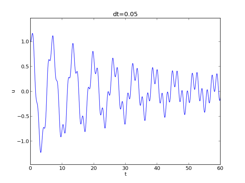
(31). As a demo of vib.py, we consider the case
\( I=1 \), \( V=0 \), \( m=1 \), \( c=0.03 \), \( s(u)=\sin(u) \), \( F(t)=3\cos(4t) \),
\( \Delta t = 0.05 \), and \( T=140 \). The relevant command to run is
Terminal> python vib.py --s 'sin(u)' --F '3*cos(4*t)' --c 0.03
This results in a moving window following the function on the screen. Figure 11 shows a part of the time series.
Figure 11: Damped oscillator excited by a sinusoidal function.
The Euler-Cromer scheme for the generalized model
The ideas of the Euler-Cromer method from the section The Euler-Cromer method carry over to the generalized model. We write (31) as two equations for \( u \) and \( v=u^{\prime} \). The first equation is taken as the one with \( v' \) on the left-hand side: $$ \begin{align} v' &= \frac{1}{m}(F(t)-s(u)-f(v)), \tag{42}\\ u^{\prime} &= v\tp \tag{43} \end{align} $$ The idea is to step (42) forward using a standard Forward Euler method, while we update \( u \) from (43) with a Backward Euler method, utilizing the recent, computed \( v^{n+1} \) value. In detail, $$ \begin{align} \frac{v^{n+1}-v^n}{\Delta t} &= \frac{1}{m}(F(t_n)-s(u^n)-f(v^n)), \tag{44}\\ \frac{u^{n+1}-u^n}{\Delta t} &= v^{n+1}, \tag{47} \end{align} $$ resulting in the explicit scheme $$ \begin{align} v^{n+1} &= v^n + \Delta t\frac{1}{m}(F(t_n)-s(u^n)-f(v^n)), \tag{46}\\ u^{n+1} &= u^n + \Delta t\,v^{n+1}\tp \tag{47} \end{align} $$ We immediately note one very favorable feature of this scheme: all the nonlinearities in \( s(u) \) and \( f(v) \) are evaluated at a previous time level. This makes the Euler-Cromer method easier to apply and hence much more convenient than the centered scheme for the second-order ODE (31).
The initial conditions are trivially set as $$ \begin{align} v^0 &= V, \\ u^0 &= I\tp \end{align} $$
Exercises and Problems
Problem 1: Use linear/quadratic functions for verification
Consider the ODE problem $$ u^{\prime\prime} + \omega^2u=f(t), \quad u(0)=I,\ u^{\prime}(0)=V,\ t\in(0,T]\tp$$ Discretize this equation according to \( [D_tD_t u + \omega^2 u = f]^n \).
a) Derive the equation for the first time step (\( u^1 \)).
b) For verification purposes, we use the method of manufactured solutions (MMS) with the choice of \( \uex(x,t)= ct+d \). Find restrictions on \( c \) and \( d \) from the initial conditions. Compute the corresponding source term \( f \) by term. Show that \( [D_tD_t t]^n=0 \) and use the fact that the \( D_tD_t \) operator is linear, \( [D_tD_t (ct+d)]^n = c[D_tD_t t]^n + [D_tD_t d]^n = 0 \), to show that \( \uex \) is also a perfect solution of the discrete equations.
c)
Use sympy to do the symbolic calculations above. Here is a
sketch of the program vib_undamped_verify_mms.py:
import sympy as sp
V, t, I, w, dt = sp.symbols('V t I w dt')  # global symbols
f = None  # global variable for the source term in the ODE

def ode_source_term(u):
    """Return the terms in the ODE that the source term
    must balance, here u'' + w**2*u.
    u is symbolic Python function of t."""
    return sp.diff(u(t), t, t) + w**2*u(t)

def residual_discrete_eq(u):
    """Return the residual of the discrete eq. with u inserted."""
    R = ...
    return sp.simplify(R)

def residual_discrete_eq_step1(u):
    """Return the residual of the discrete eq. at the first
    step with u inserted."""
    R = ...
    return sp.simplify(R)

def DtDt(u, dt):
    """Return 2nd-order finite difference for u_tt.
    u is a symbolic Python function of t.
    """
    return ...

def main(u):
    """
    Given some chosen solution u (as a function of t, implemented
    as a Python function), use the method of manufactured solutions
    to compute the source term f, and check if u also solves
    the discrete equations.
    """
    print '=== Testing exact solution: %s ===' % u
    print "Initial conditions u(0)=%s, u'(0)=%s:" % \
          (u(t).subs(t, 0), sp.diff(u(t), t).subs(t, 0))

    # Method of manufactured solution requires fitting f
    global f  # source term in the ODE
    f = sp.simplify(ode_lhs(u))

    # Residual in discrete equations (should be 0)
    print 'residual step1:', residual_discrete_eq_step1(u)
    print 'residual:', residual_discrete_eq(u)

def linear():
    main(lambda t: V*t + I)

if __name__ == '__main__':
    linear()
Fill in the various functions such that the calls in the main
function works.
d)
The purpose now is to choose a quadratic function
\( \uex = bt^2 + ct + d \) as exact solution. Extend the sympy
code above with a function quadratic for fitting f and checking
if the discrete equations are fulfilled. (The function is very similar
to linear.)
e) Will a polynomial of degree three fulfill the discrete equations?
f)
Implement a solver function for computing the numerical
solution of this problem.
g)
Write a nose test for checking that the quadratic solution
is computed to correctly (too machine precision, but the
round-off errors accumulate and increase with \( T \)) by the solver
function.
Filenames: vib_undamped_verify_mms.pdf, vib_undamped_verify_mms.py.
Exercise 2: Show linear growth of the phase with time
Consider an exact solution \( I\cos (\omega t) \) and an
approximation \( I\cos(\tilde\omega t) \).
Define the phase error as time lag between the peak \( I \)
in the exact solution and the corresponding peak in the approximation
after \( m \) periods of oscillations. Show that this phase error
is linear in \( m \).
Filename: vib_phase_error_growth.pdf.
Exercise 3: Improve the accuracy by adjusting the frequency
According to (11), the numerical
frequency deviates from the exact frequency by a (dominating) amount
\( \omega^3\Delta t^2/24 >0 \). Replace the w parameter in the algorithm
in the solver function in vib_undamped.py by w*(1 -
(1./24)*w**2*dt**2 and test how this adjustment in the numerical
algorithm improves the accuracy (use \( \Delta t =0.1 \) and simulate
for 80 periods, with and without adjustment of \( \omega \)).
Filename: vib_adjust_w.py.
Exercise 4: See if adaptive methods improve the phase error
Adaptive methods for solving ODEs aim at adjusting \( \Delta t \) such
that the error is within a user-prescribed tolerance. Implement the
equation \( u^{\prime\prime}+u=0 \) in the Odespy
software. Use the example on adaptive
schemes
in [1]. Run the scheme with a very low
tolerance (say \( 10^{-14} \)) and for a long time, check the number of
time points in the solver's mesh (len(solver.t_all)), and compare
the phase error with that produced by the simple finite difference
method from the section A centered finite difference scheme with the same number of (equally
spaced) mesh points. The question is whether it pays off to use an
adaptive solver or if equally many points with a simple method gives
about the same accuracy.
Filename: vib_undamped_adaptive.py.
Exercise 5: Use a Taylor polynomial to compute \( u^1 \)
As an alternative to the derivation of (8) for
computing \( u^1 \), one can use a Taylor polynomial with three terms
for \( u^1 \):
$$ u(t_1) \approx u(0) + u^{\prime}(0)\Delta t + {\half}u^{\prime\prime}(0)\Delta t^2$$
With \( u^{\prime\prime}=-\omega^2 u \) and \( u^{\prime}(0)=0 \), show that this method also leads to
(8). Generalize the condition on \( u^{\prime}(0) \) to
be \( u^{\prime}(0)=V \) and compute \( u^1 \) in this case with both methods.
Filename: vib_first_step.pdf.
Exercise 6: Find the minimal resolution of an oscillatory function
Sketch the function on a given mesh which has the highest possible
frequency. That is, this oscillatory "cos-like" function has its
maxima and minima at every two grid points. Find an expression for
the frequency of this function, and use the result to find the largest
relevant value of \( \omega\Delta t \) when \( \omega \) is the frequency
of an oscillating function and \( \Delta t \) is the mesh spacing.
Filename: vib_largest_wdt.pdf.
Exercise 7: Visualize the accuracy of finite differences for a cosine function
We introduce the error fraction
$$ E = \frac{[D_tD_t u]^n}{u^{\prime\prime}(t_n)} $$
to measure the error in the finite difference approximation \( D_tD_tu \) to
\( u^{\prime\prime} \).
Compute \( E \)
for the specific choice of a cosine/sine function of the
form \( u=\exp{(i\omega t)} \) and show that
$$ E = \left(\frac{2}{\omega\Delta t}\right)^2
\sin^2(\frac{\omega\Delta t}{2})
\tp
$$
Plot \( E \) as a function of \( p=\omega\Delta t \). The relevant
values of \( p \) are \( [0,\pi] \) (see Exercise 6: Find the minimal resolution of an oscillatory function
for why \( p>\pi \) does not make sense).
The deviation of the curve from unity visualizes the error in the
approximation. Also expand \( E \) as a Taylor polynomial in \( p \) up to
fourth degree (use, e.g., sympy).
Filename: vib_plot_fd_exp_error.py.
Exercise 8: Verify convergence rates of the error in energy
We consider the ODE problem \( u^{\prime\prime} + \omega^2u=0 \), \( u(0)=I \), \( u^{\prime}(0)=V \), for \( t\in (0,T] \). The total energy of the solution \( E(t)=\half(u^{\prime})^2 + \half\omega^2 u^2 \) should stay constant. The error in energy can be computed as explained in the section Energy considerations.
Make a nose test in a file test_error_conv.py, where code from
vib_undamped.py is imported, but the convergence_rates and
test_convergence_rates functions are copied and modified to also
incorporate computations of the error in energy and the convergence
rate of this error. The expected rate is 2.
Filename: test_error_conv.py.
Exercise 9: Use linear/quadratic functions for verification
This exercise is a generalization of Problem 1: Use linear/quadratic functions for verification to the extended model problem
(31) where the damping term is either linear or quadratic.
Solve the various subproblems and see how the results and problem
settings change with the generalized ODE in case of linear or
quadratic damping. By modifying the code from Problem 1: Use linear/quadratic functions for verification, sympy will do most
of the work required to analyze the generalized problem.
Filename: vib_verify_mms.py.
Exercise 10: Use an exact discrete solution for verification
Write a nose test function in a separate file
that employs the exact discrete solution
(12) to verify the implementation of the
solver function in the file vib_undamped.py.
Filename: test_vib_undamped_exact_discrete_sol.py.
Exercise 11: Use analytical solution for convergence rate tests
The purpose of this exercise is to perform convergence tests of the
problem (31) when \( s(u)=\omega^2u \) and \( F(t)=A\sin\phi t \).
Find the complete analytical solution to the problem in this case
(most textbooks on mechanics or ordinary differential equations list
the various elements you need to write down the exact solution).
Modify the convergence_rate function from the vib_undamped.py
program to perform experiments with the extended model. Verify that
the error is of order \( \Delta t^2 \).
Filename: vib_conv_rate.py.
Exercise 12: Investigate the amplitude errors of many solvers
Use the program vib_undamped_odespy.py from the section Standard methods for 1st-order ODE systems
and the amplitude estimation from the amplitudes function
in the vib_undamped.py file (see the section Empirical analysis of the solution)
to investigate how well famous methods for 1st-order ODEs
can preserve the amplitude of \( u \) in undamped oscillations.
Test, for example, the 3rd- and 4th-order Runge-Kutta methods
(RK3, RK4), the Crank-Nicolson method (CrankNicolson),
the 2nd- and 3rd-order Adams-Bashforth methods (AdamsBashforth2,
AdamsBashforth3), and a 2nd-order Backwards scheme (Backward2Step).
The relevant governing equations are listed in
the section ref{vib:model2x2:ueq}.
Filename: vib_amplitude_errors.py.
Exercise 13: Minimize memory usage of a vibration solver
The program vib.py
store the complete solution \( u^0,u^1,\ldots,u^{N_t} \) in memory, which is
convenient for later plotting.
Make a memory minimizing version of this program where only the last three
\( u^{n+1} \), \( u^n \), and \( u^{n-1} \) values are stored in memory.
Write each computed \( (t_{n+1}, u^{n+1}) \) pair to file.
Visualize the data in the file (a cool solution is to
read one line at a time and
plot the \( u \) value using the line-by-line plotter in the
visualize_front_ascii function - this technique makes it trivial
to visualize very long time simulations).
Filename: vib_memsave.py.
Exercise 14: Implement the solver via classes
Reimplement the vib.py
program
using a class Problem to hold all the physical parameters of the problem,
a class Solver to hold the numerical parameters and compute the
solution, and a class Visualizer to display the solution.
Hint.
Use the ideas and examples
for an ODE model.
More specifically, make a superclass Problem for holding the scalar
physical parameters of a problem and let subclasses implement the
\( s(u) \) and \( F(t) \) functions as methods.
Try to call up as much existing functionality in vib.py as possible.
Filename: vib_class.py.
Exercise 15: Interpret \( [D_tD_t u]^n \) as a forward-backward difference
Show that the difference \( [D_t D_tu]^n \) is equal to \( [D_t^+D_t^-u]^n \)
and \( D_t^-D_t^+u]^n \). That is, instead of applying a centered difference
twice one can alternatively apply a mixture forward and backward
differences.
Filename: vib_DtDt_fw_bw.pdf.
Exercise 16: Use the forward-backward scheme with quadratic damping
We consider the generalized model with quadratic damping, expressed as a system of two first-order equations as in the section ref{vib:ode2:staggered}: $$ \begin{align*} u^{\prime} &= v,\\ v' &= \frac{1}{m}\left( F(t) - \beta |v|v - s(u)\right)\tp \end{align*} $$ However, contrary to what is done in the section ref{vib:ode2:staggered}, we want to apply the idea of the forward-backward discretization in the section The Euler-Cromer method. Express the idea in operator notation and write out the scheme. Unfortunately, the backward difference for the \( v \) equation creates a nonlinearity \( |v^{n+1}|v^{n} \). To linearize this nonlinearity, use the known value \( v^n \) inside the absolute value factor, i.e., \( |v^{n+1}|v^{n}\approx |v^n|v^{n+1} \). Show that the resulting scheme is equivalent to the one in the section ref{vib:ode2:staggered} for some time level \( n\geq 1 \).
What we learn from this exercise is that the first-order differences
and the linearization trick play together in "the right way" such that
the scheme is as good as when we (in the section ref{vib:ode2:staggered})
carefully apply centered differences and a geometric mean on a
staggered mesh to achieve second-order accuracy. There is a
difference in the handling of the initial conditions, though, as
explained at the end of the section The Euler-Cromer method.
Filename: vib_gen_bwdamping.pdf.
Exercise 17: Use a backward difference for the damping term
As an alternative to discretizing the damping terms \( \beta u^{\prime} \) and
\( \beta |u^{\prime}|u^{\prime} \) by centered differences, we may apply
backward differences:
$$
\begin{align*}
[u^{\prime}]^n &\approx [D_t^-u]^n,\\
& [|u^{\prime}|u^{\prime}]^n &\approx [|D_t^-u|D_t^-u]^n
= |[D_t^-u]^n|[D_t^-u]^n\tp
\end{align*}
$$
The advantage of the backward difference is that the damping term is
evaluated using known values \( u^n \) and \( u^{n-1} \) only.
Extend the vib.py code with a scheme based
on using backward differences in the damping terms. Add statements
to compare the original approach with centered difference and the
new idea launched in this exercise. Perform numerical experiments
to investigate how much accuracy that is lost by using the backward
differences.
Filename: vib_gen_bwdamping.pdf.
Exercise 18: Simulate a bouncing ball
A bouncing ball is a body in free vertically fall until it impacts the ground. During the impact, some kinetic energy is lost, and a new motion upwards with reduced velocity starts. At some point the velocity close to the ground is so small that the ball is considered to be finally at rest.
The motion of the ball falling in air is governed by Newton's second law \( F=ma \), where \( a \) is the acceleration of the body, \( m \) is the mass, and \( F \) is the sum of all forces. Here, we neglect the air resistance so that gravity \( -mg \) is the only force. The height of the ball is denoted by \( h \) and \( v \) is the velocity. The relations between \( h \), \( v \), and \( a \), $$ h'(t)= v(t),\quad v'(t) = a(t),$$ combined with Newton's second law gives the ODE model $$ \begin{equation} h^{\prime\prime}(t) = -g, \tag{48} \end{equation} $$ or expressed alternatively as a system of first-order equations: $$ \begin{align} v'(t) &= -g, \tag{49} \\ h'(t) &= v(t)\tp \tag{50} \end{align} $$ These equations govern the motion as long as the ball is away from the ground by a small distance \( \epsilon_h > 0 \). When \( h < \epsilon_h \), we have two cases.
- The ball impacts the ground, recognized by a sufficiently large negative velocity (\( v < -\epsilon_v \)). The velocity then changes sign and is reduced by a factor \( C_R \), known as the coefficient of restitution. For plotting purposes, one may set \( h=0 \).
- The motion stops, recognized by a sufficiently small velocity (\( |v| < \epsilon_v \)) close to the ground.
Hint. A naive implementation may get stuck in repeated impacts for large time step sizes. To avoid this situation, one can introduce a state variable that holds the mode of the motion: free fall, impact, or rest. Two consecutive impacts imply that the motion has stopped.
Filename: bouncing_ball.py.
Exercise 19: Simulate an elastic pendulum
Consider an elastic pendulum fixed to the point \( \boldsymbol{r}_0=(0,L_0) \). The length of the pendulum wire when not stretched is \( L_0 \). The wire is massless and always straight. At the end point \( \boldsymbol{r} \), we have a mass \( m \). Stretching the elastic wire a distance \( s \) gives rise to a spring force \( ks \) in the opposite direction of the stretching. Let \( \boldsymbol{n} \) be a unit normal vector along the wire: $$ \boldsymbol{n} = \frac{\boldsymbol{r}-\boldsymbol{r}_0}{||\boldsymbol{r}-\boldsymbol{r}_0||}\tp$$ The stretch \( s \) in the wire is the current length \( ||\boldsymbol{r}-\boldsymbol{r}_0|| \) at some time \( t \) minus the original length \( L_0 \): $$ s = ||\boldsymbol{r}-\boldsymbol{r}_0|| - L_0\tp$$ The force in the wire is then \( \boldsymbol{F}_w=-ks\boldsymbol{n} \). Newton's second law of motion applied to the mass results in $$ \begin{equation} m\ddot{\boldsymbol{r}} = -ks\boldsymbol{n} - mg\boldsymbol{j}, \tag{51} \end{equation} $$ where \( \boldsymbol{j} \) is a unit vector in the upward vertical direction. Let \( \boldsymbol{r}=(x,y) \) and \( \boldsymbol{n}=(n_x,n_y) \). The two components of (51) then becomes $$ \begin{align} \ddot x &= -m^{-1}ksn_x,\\ \tag{52} \\ \ddot y &= - m^{-1}ksn_y - g \tag{53}\tp \end{align} $$ The mass point \( (x,y) \) will undergo a two-dimensional motion, but if the wire is stiff (large \( k \)), the elastic pendulum will approach the classical one where the mass point moves along a circle. However, the elastic pendulum is modeled by a direct application of Newton's second law, because the force in the wire is known (as a function of the motion), while the classical pendulum involves constrained motion, which requires elimination of an unknown via the constraint (by invoking polar coordinates).
In equilibrium, the mass hangs in the position \( (0,y_0) \) determined by $$ 0 = - m^{-1}ksn_y - g = m^{-1}k(y_0-L_0) - g\quad\Rightarrow\quad y_0 = L_0 + mg/k = L\tp$$ We then displace the mass an angle \( \theta_0 \) to the right. The initial position \( (x(0),y(0)) \) then becomes $$ x(0)=L\sin\theta_0,\quad y(0)=L_0 - L\cos\theta_0\tp$$ The velocity is zero, \( x'(0)=y'(0)=0 \).
a) Write a code that can simulate such an elastic pendulum. Plot \( y \) against \( x \) in a plot with the same length scale on the axis such that we get a correct picture of the motion. Also plot the angle the pendulum: \( \theta = \tan^{-1}x/(L_0-y) \).
A possible set of parameters is \( L_0=9.81 \) m, \( m=1 \) kg, \( theta_0=30 \) degrees.
Hint 1. The associated classical pendulum, for large \( k \), has an equation \( \ddot\theta + g/L_0\theta =0 \). With \( g=L_0 \), the period is \( 2\pi \): \( \theta(t) = \theta_0\cos(t) \). One can compare in a plot the angle of the elastic solution (\( \theta = \tan^{-1}x/(L_0-y) \)) with the solution of the classical pendulum problem.
Hint 2. The equation of motion is subject to round-off errors for large \( k \), because \( s \) is then small such that \( ks \) is a product of a large and a small number. Moreover, in this stiff case, \( m^{-1}ksn_y \) is close to \( g \) such that we also subtract two almost equal numbers in the force term in the equation. For the given parameters, \( k=150 \) is a large value and gives a solution close to the motion of a perfect classical pendulum. Much larger values gives unstable solutions.
b) Air resistance is a force \( \frac{1}{2}\varrho C_D A||bm{v}||\boldsymbol{v} \), where \( C_D \) is a drag coefficient (0.2 for a sphere), \( \varrho \) is the density of air (1.2 \( \hbox{kg }\,{\hbox{m}}^{-3} \)), \( A \) is the cross section area (\( A=\pi R^2 \) for a sphere, where \( R \) is the radius), and \( \boldsymbol{v} \) is the velocity: \( \boldsymbol{v} = \dot{\boldsymbol{r}} \). Include air resistance in the model and show plots comparing the motion with and without air resistance.
Filename: elastic_pendulum.py.
Exercise 20: Analysis of the Euler-Cromer scheme
The Euler-Cromer scheme for the model problem \( u^{\prime\prime} + \omega^2 u =0 \), \( u(0)=I \), \( u^{\prime}(0)=0 \), is given in (27)-(26). Find the exact discrete solutions of this scheme and show that the solution for \( u^n \) coincides with that found in the section Analysis of the numerical scheme.
Hint. Use an "ansatz" \( u^n=I\exp{(i\tilde\omega\Delta t\,n)} \) and \( v^=qu^n \), where \( \tilde\omega \) and \( q \) are unknown parameters. The formula $$ \exp{(i\tilde\omega(\Delta t))} + \exp{(i\tilde\omega(-\Delta t))} - 2 = 2\left(\cosh(i\tilde\omega\Delta t) -1 \right) =-4\sin^2(\frac{\tilde\omega\Delta t}{2}),$$ becomes handy.
References
- H. P. Langtangen. Introduction to Computing With Finite Difference Methods, Simula Research Laboratory and University of Oslo, 2013, http://hplgit.github.com/INF5620/doc/notes/decay-sphinx/main_decay.html.