$$ \newcommand{\uex}{{u_{\small\mbox{e}}}} \newcommand{\tp}{\thinspace .} $$

Study Guide: Scientific software engineering for a simple ODE problem

Hans Petter Langtangen [1, 2]

[1] Center for Biomedical Computing, Simula Research Laboratory [2] Department of Informatics, University of Oslo

Sep 25, 2014

Creating user interfaces
Accessing command-line arguments
Reading a sequence of command-line arguments
Implementation
Working with an argument parser
Reading option-values pairs
A graphical user interface
The Parampool package
Making a compute function
The hard part of the compute function: the HTML code
How to embed a PNG plot in HTML code
Generating the user interface
Running the web application
More advanced use
Computing convergence rates
Estimating the convergence rate $ r $
Implementation
Execution
Debugging via convergence rates
Software engineering
Making a module
Sketch of the module
Test block
Extended test block
Prefixing imported functions by the module name
Downside of module prefix notation
Doctests
Running doctests
Unit testing with nose
Basic use of nose
Example on a nose test in the source code
Example on a nose test in a separate file
The habit of writing nose tests
Purpose of a test function: raise AssertionError if failure
Advantages of nose
Demonstrating nose (ideas)
Demonstrating nose (code)
Floats as test results require careful comparison
Test of wrong use
Test of convergence rates
Classical unit testing with unittest
Basic use of unittest
Demonstration of unittest
Implementing simple problem and solver classes
What to learn
The problem class
Improved problem class
The solver class
The visualizer class
Combing the classes
Implementing more advanced problem and solver classes
A generic class for parameters
The problem class
The solver class
The visualizer class
Performing scientific experiments
Model problem and numerical solution method
Plan for the experiments
Typical plot summarizing the results
Script code
Comments to the code
Interpreting output from other programs
Code for grabbing output from another program
Code for interpreting the grabbed output
Making a report
Publishing a complete project

Creating user interfaces

Never edit the program to change input!

Set input data on the command line or in a graphical user interface

How is explained next

Accessing command-line arguments

All command-line arguments are available in sys.argv

sys.argv[0] is the program

sys.argv[1:] holds the command-line arguments

Method 1: fixed sequence of parameters on the command line

Method 2: --option value pairs on the command line (with default values)

Terminal> python myprog.py 1.5 2 0.5 0.8 0.4
Terminal> python myprog.py --I 1.5 --a 2 --dt 0.8 0.4

Reading a sequence of command-line arguments

The program decay_plot.py needs this input:

$ I $

$ a $

$ T $

an option to turn the plot on or off (makeplot)

a list of $ \Delta t $ values

Give these on the command line in correct sequence

Terminal> python decay_cml.py 1.5 2 0.5 0.8 0.4

Implementation

import sys

def read_command_line():
    if len(sys.argv) < 6:
        print 'Usage: %s I a T on/off dt1 dt2 dt3 ...' % \ 
              sys.argv[0]; sys.exit(1)  # abort

    I = float(sys.argv[1])
    a = float(sys.argv[2])
    T = float(sys.argv[3])
    makeplot = sys.argv[4] in ('on', 'True')
    dt_values = [float(arg) for arg in sys.argv[5:]]

    return I, a, T, makeplot, dt_values

Note:

sys.argv[i] is always a string

Must explicitly convert to (e.g.) float for computations

List comprehensions make lists: [expression for e in somelist]

Complete program: decay_cml.py.

Working with an argument parser

Set option-value pairs on the command line if the default value is not suitable:

Terminal> python decay_argparse.py --I 1.5 --a 2 --dt 0.8 0.4

Code:

def define_command_line_options():
    import argparse
    parser = argparse.ArgumentParser()
    parser.add_argument('--I', '--initial_condition', type=float,
                        default=1.0, help='initial condition, u(0)',
                        metavar='I')
    parser.add_argument('--a', type=float,
                        default=1.0, help='coefficient in ODE',
                        metavar='a')
    parser.add_argument('--T', '--stop_time', type=float,
                        default=1.0, help='end time of simulation',
                        metavar='T')
    parser.add_argument('--makeplot', action='store_true',
                        help='display plot or not')
    parser.add_argument('--dt', '--time_step_values', type=float,
                        default=[1.0], help='time step values',
                        metavar='dt', nargs='+', dest='dt_values')
    return parser

(metavar is the symbol used in help output)

Reading option-values pairs

argparse.ArgumentParser parses the command-line arguments:

def read_command_line():
    parser = define_command_line_options()
    args = parser.parse_args()
    print 'I={}, a={}, T={}, makeplot={}, dt_values={}'.format(
        args.I, args.a, args.T, args.makeplot, args.dt_values)
    return args.I, args.a, args.T, args.makeplot, args.dt_values

Complete program: decay_argparse.py.

A graphical user interface

Normally very much programming required - and much competence on graphical user interfaces.

Here: use a tool to automatically create it in a few minutes (!)

The Parampool package

Parampool is a package for handling a large pool of input parameters in simulation programs

Parampool can automatically create a sophisticated web-based graphical user interface (GUI) to set parameters and view solutions

Remark.

The forthcoming material aims at those with particular interest in equipping their programs with a GUI - others can safely skip it.

Making a compute function

Key concept: a compute function that takes all input data as arguments and returning HTML code for viewing the results (e.g., plots and numbers)

What we have: decay_plot.py

main function carries out simulations and plotting for a series of $ \Delta t $ values

Goal: steer and view these experiments from a web GUI

What to do:

create a compute function

call parampool functionality

The compute function main_GUI:

def main_GUI(I=1.0, a=.2, T=4.0,
         dt_values=[1.25, 0.75, 0.5, 0.1],
         theta_values=[0, 0.5, 1]):

The hard part of the compute function: the HTML code

The results are to be displayed in a web page

Only you know what to display in your problem

Therefore, you need to specify the HTML code

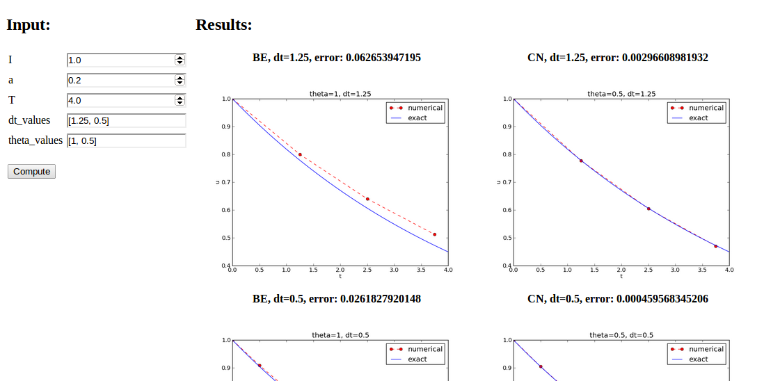
Suppose explore solves the problem, makes a plot, computes the error and returns appropriate HTML code with the plot. Embed error and plots in a table:

def main_GUI(I=1.0, a=.2, T=4.0,
         dt_values=[1.25, 0.75, 0.5, 0.1],
         theta_values=[0, 0.5, 1]):
    # Build HTML code for web page. Arrange plots in columns
    # corresponding to the theta values, with dt down the rows
    theta2name = {0: 'FE', 1: 'BE', 0.5: 'CN'}
    html_text = '<table>\n'
    for dt in dt_values:
        html_text += '<tr>\n'
        for theta in theta_values:
            E, html = explore(I, a, T, dt, theta, makeplot=True)
            html_text += """
<td>
<center><b>%s, dt=%g, error: %s</b></center><br>
%s
</td>
""" % (theta2name[theta], dt, E, html)
        html_text += '</tr>\n'
    html_text += '</table>\n'
    return html_text

How to embed a PNG plot in HTML code

In explore:

import matplotlib.pyplot as plt
...
# plot
plt.plot(t, u, r-')
plt.xlabel('t')
plt.ylabel('u')
...
from parampool.utils import save_png_to_str
html_text = save_png_to_str(plt, plotwidth=400)

If you know HTML, you can return more sophisticated layout etc.

Generating the user interface

Make a file decay_GUI_generate.py:

from parampool.generator.flask import generate
from decay_GUI import main
generate(main,
         output_controller='decay_GUI_controller.py',
         output_template='decay_GUI_view.py',
         output_model='decay_GUI_model.py')

Running decay_GUI_generate.py results in

decay_GUI_model.py defines HTML widgets to be used to set input data in the web interface,

templates/decay_GUI_views.py defines the layout of the web page,

decay_GUI_controller.py runs the web application.

Good news: we only need to run decay_GUI_controller.py and there is no need to look into any of these files!

Running the web application

Start the GUI

Terminal> python decay_GUI_controller.py

Open a web browser at 127.0.0.1:5000

More advanced use

The compute function can have arguments of type float, int, string, list, dict, numpy array, filename (file upload)

Alternative: specify a hierarchy of input parameters with name, default value, data type, widget type, unit (m, kg, s), validity check

The generated web GUI can have user accounts with login and storage of results in a database

Computing convergence rates

Frequent assumption on the relation between the numerical error $ E $ and some discretization parameter $ \Delta t $: $$ \begin{equation} E = C\Delta t^r, \label{decay:E:dt} \end{equation} $$

Unknown: $ C $ and $ r $.

Goal: estimate $ r $ (and $ C $) from numerical experiments

Estimating the convergence rate $ r $

Perform numerical experiments: $ (\Delta t_i, E_i) $, $ i=0,\ldots,m-1 $. Two methods for finding $ r $ (and $ C $):

Take the logarithm of \eqref{decay:E:dt}, $ \ln E = r\ln \Delta t + \ln C $, and fit a straight line to the data points $ (\Delta t_i, E_i) $, $ i=0,\ldots,m-1 $.

Consider two consecutive experiments, $ (\Delta t_i, E_i) $ and $ (\Delta t_{i-1}, E_{i-1}) $. Dividing the equation $ E_{i-1}=C\Delta t_{i-1}^r $ by $ E_{i}=C\Delta t_{i}^r $ and solving for $ r $ yields

$$ \begin{equation} r_{i-1} = \frac{\ln (E_{i-1}/E_i)}{\ln (\Delta t_{i-1}/\Delta t_i)} \label{decay:conv:rate} \end{equation} $$ for $ i=1,=\ldots,m-1 $.

Method 2 is best.

Implementation

Compute $ r_0, r_1, \ldots, r_{m-2} $:

from math import log

def main():
    I, a, T, makeplot, dt_values = read_command_line()
    r = {}  # estimated convergence rates
    for theta in 0, 0.5, 1:
        E_values = []
        for dt in dt_values:
            E = explore(I, a, T, dt, theta, makeplot=False)
            E_values.append(E)

        # Compute convergence rates
        m = len(dt_values)
        r[theta] = [log(E_values[i-1]/E_values[i])/
                    log(dt_values[i-1]/dt_values[i])
                    for i in range(1, m, 1)]

    for theta in r:
        print '\nPairwise convergence rates for theta=%g:' % theta
        print ' '.join(['%.2f' % r_ for r_ in r[theta]])
    return r

Complete program: decay_convrate.py.

Execution

Terminal> python decay_convrate.py --dt 0.5 0.25 0.1 0.05 0.025 0.01
...
Pairwise convergence rates for theta=0:
1.33 1.15 1.07 1.03 1.02

Pairwise convergence rates for theta=0.5:
2.14 2.07 2.03 2.01 2.01

Pairwise convergence rates for theta=1:
0.98 0.99 0.99 1.00 1.00

Strong verification method.

Verify that $ r $ has the expected value!

Debugging via convergence rates

Potential bug: missing a in the denominator,

u[n+1] = (1 - (1-theta)*a*dt)/(1 + theta*dt)*u[n]

Running decay_convrate.py gives same rates.

Why? The value of $ a $... ($ a=1 $)

0 and 1 are bad values in tests!

Better:

Terminal> python decay_convrate.py --a 2.1 --I 0.1  \ 
          --dt 0.5 0.25 0.1 0.05 0.025 0.01
...
Pairwise convergence rates for theta=0:
1.49 1.18 1.07 1.04 1.02

Pairwise convergence rates for theta=0.5:
-1.42 -0.22 -0.07 -0.03 -0.01

Pairwise convergence rates for theta=1:
0.21 0.12 0.06 0.03 0.01

Forward Euler works...because $ \theta=0 $ hides the bug.

This bug gives $ r\approx 0 $:

u[n+1] = ((1-theta)*a*dt)/(1 + theta*dt*a)*u[n]

Software engineering

Goal: make more professional numerical software.

Topics:

How to make modules (reusable libraries)

Testing frameworks (doctest, nose, unittest)

Implementation with classes

Making a module

Previous programs: much repetitive code (esp. solver)

DRY (Don't Repeat Yourself) principle: no copies of code

A change needs to be done in one and only one place

Module = just a file with functions (reused through import)

Let's make a module by putting these functions in a file:

solver

verify_three_steps

verify_discrete_solution

explore

define_command_line_options

read_command_line

main (with convergence rates)

verify_convergence_rate

Module name: decay_mod, filename: decay_mod.py.

Sketch of the module

from numpy import *
from matplotlib.pyplot import *
import sys

def solver(I, a, T, dt, theta):
    ...

def verify_three_steps():
    ...

def verify_exact_discrete_solution():
    ...

def u_exact(t, I, a):
    ...

def explore(I, a, T, dt, theta=0.5, makeplot=True):
    ...

def define_command_line_options():
    ...

def read_command_line(use_argparse=True):
    ...

def main():
    ...

That is! It's a module decay_mod in file decay_mod.py.

Usage in some other program:

from decay_mod import solver
u, t = solver(I=1.0, a=3.0, T=3, dt=0.01, theta=0.5)

Test block

At the end of a module it is common to include a test block:

if __name__ == '__main__':
    main()

Note:

If decay_mod is imported, __name__ is decay_mod.

If decay_mod.py is run, __name__ is __main__.

Use test block for testing, demo, user interface, ...

Extended test block

if __name__ == '__main__':
    if 'verify' in sys.argv:
        if verify_three_steps() and verify_discrete_solution():
            pass # ok
        else:
            print 'Bug in the implementation!'
    elif 'verify_rates' in sys.argv:
        sys.argv.remove('verify_rates')
        if not '--dt' in sys.argv:
            print 'Must assign several dt values'
            sys.exit(1)  # abort
        if verify_convergence_rate():
            pass
        else:
            print 'Bug in the implementation!'
    else:
        # Perform simulations
        main()

Prefixing imported functions by the module name

from numpy import *
from matplotlib.pyplot import *

This imports a large number of names (sin, exp, linspace, plot, ...).

Confusion: is a function from numpy? Or matplotlib.pyplot?

Alternative (recommended) import:

import numpy
import matplotlib.pyplot

Now we need to prefix functions with module name:

t = numpy.linspace(0, T, Nt+1)
u_e = I*numpy.exp(-a*t)
matplotlib.pyplot.plot(t, u_e)

Common standard:

import numpy as np
import matplotlib.pyplot as plt

t = np.linspace(0, T, Nt+1)
u_e = I*np.exp(-a*t)
plt.plot(t, u_e)

Downside of module prefix notation

A math line like $ e^{-at}\sin(2\pi t) $ gets cluttered with module names,

numpy.exp(-a*t)*numpy.sin(2(numpy.pi*t)
# or
np.exp(-a*t)*np.sin(2*np.pi*t)

Solution (much used in this course): do two imports

import numpy as np
from numpy import exp, sin, pi
...
t = np.linspace(0, T, Nt+1)
u_e = exp(-a*t)*sin(2*pi*t)

Doctests

Doc strings can be equipped with interactive Python sessions for demonstrating usage and automatic testing of functions.

def solver(I, a, T, dt, theta):
    """
    Solve u'=-a*u, u(0)=I, for t in (0,T] with steps of dt.


    >>> u, t = solver(I=0.8, a=1.2, T=4, dt=0.5, theta=0.5)
    >>> for t_n, u_n in zip(t, u):
    ...     print 't=%.1f, u=%.14f' % (t_n, u_n)
    t=0.0, u=0.80000000000000
    t=0.5, u=0.43076923076923
    t=1.0, u=0.23195266272189
    t=1.5, u=0.12489758761948
    t=2.0, u=0.06725254717972
    t=2.5, u=0.03621291001985
    t=3.0, u=0.01949925924146
    t=3.5, u=0.01049960113002
    t=4.0, u=0.00565363137770
    """
    ...

Running doctests

Automatic check that the code reproduces the doctest output:

Terminal> python -m doctest decay_mod_doctest.py

Report in case of failure:

Terminal> python -m doctest decay_mod_doctest.py
********************************************************
File "decay_mod_doctest.py", line 12, in decay_mod_doctest....
Failed example:
    for t_n, u_n in zip(t, u):
        print 't=%.1f, u=%.14f' % (t_n, u_n)
Expected:
    t=0.0, u=0.80000000000000
    t=0.5, u=0.43076923076923
    t=1.0, u=0.23195266272189
    t=1.5, u=0.12489758761948
    t=2.0, u=0.06725254717972
Got:
    t=0.0, u=0.80000000000000
    t=0.5, u=0.43076923076923
    t=1.0, u=0.23195266272189
    t=1.5, u=0.12489758761948
    t=2.0, u=0.06725254718756
********************************************************
1 items had failures:
   1 of   2 in decay_mod_doctest.solver
***Test Failed*** 1 failures.

Floats are difficult to compare.

Limit the number of digits in the output in doctests! Otherwise, round-off errors on a different machine may ruin the test.

Complete program: decay_mod_doctest.py.

Unit testing with nose

Nose is a very user-friendly testing framework

Based on unit testing

Identify (small) units of code and test each unit

Nose automates running all tests

Good habit: run all tests after (small) edits of a code

Even better habit: write tests before the code (!)

Remark: unit testing in scientific computing is not yet well established

Basic use of nose

Implement tests in test functions with names starting with test_.

Test functions cannot have arguments.

Test functions perform assertions on computed results using assert functions from the nose.tools module.

Test functions can be in the source code files or be collected in separate files test*.py.

Example on a nose test in the source code

Very simple module mymod (in file mymod.py):

def double(n):
    return 2*n

Write test function in mymod.py:

def double(n):
    return 2*n

import nose.tools as nt

def test_double():
    result = double(4)
    nt.assert_equal(result, 8)

Running

Terminal> nosetests -s mymod

makes the nose tool run all test_*() functions in mymod.py.

Example on a nose test in a separate file

Write the test in a separate file, say test_mymod.py:

import nose.tools as nt
import mymod

def test_double():
    result = mymod.double(4)
    nt.assert_equal(result, 8)

Running

Terminal> nosetests -s

makes the nose tool run all test_*() functions in all files test*.py in the current directory and in all subdirectories (recursevely) with names tests or *_tests.

Tip.

Start with test functions in the source code file. When the file contains many tests, or when you have many source code files, move tests to separate files.

The habit of writing nose tests

Put test_*() functions in the module

When you get many test_*() functions, collect them in tests/test*.py

Purpose of a test function: raise AssertionError if failure

Alternative ways of raising AssertionError if result is not 8:

import nose.tools as nt

def test_double():
    result = ...

    nt.assert_equal(result, 8)    # alternative 1

    assert result == 8            # alternative 2

    if result != 8:               # alternative 3
        raise AssertionError()

Advantages of nose

Easier to use than other test frameworks

Tests are written and collected in a compact and structured way

Large collections of tests, scattered throughout a directory tree can be executed with one command (nosetests -s)

Nose is a much-adopted standard

Demonstrating nose (ideas)

Aim: test function solver for $ u'=-au $, $ u(0)=I $.

We design three unit tests:

A comparison between the computed $ u^n $ values and the exact discrete solution

A comparison between the computed $ u^n $ values and precomputed verified reference values

A comparison between observed and expected convergence rates

These tests follow very closely the previous verify* functions.

Demonstrating nose (code)

import nose.tools as nt
import decay_mod_unittest as decay_mod
import numpy as np

def exact_discrete_solution(n, I, a, theta, dt):
    """Return exact discrete solution of the theta scheme."""
    dt = float(dt)  # avoid integer division
    factor = (1 - (1-theta)*a*dt)/(1 + theta*dt*a)
    return I*factor**n

def test_exact_discrete_solution():
    """
    Compare result from solver against
    formula for the discrete solution.
    """
    theta = 0.8; a = 2; I = 0.1; dt = 0.8
    N = int(8/dt)  # no of steps
    u, t = decay_mod.solver(I=I, a=a, T=N*dt, dt=dt, theta=theta)
    u_de = np.array([exact_discrete_solution(n, I, a, theta, dt)
                     for n in range(N+1)])
    diff = np.abs(u_de - u).max()
    nt.assert_almost_equal(diff, 0, delta=1E-14)

Floats as test results require careful comparison

Round-off errors make exact comparison of floats unreliable

nt.assert_almost_equal: compare two floats to some digits or precision

def test_solver():
    """
    Compare result from solver against
    precomputed arrays for theta=0, 0.5, 1.
    """
    I=0.8; a=1.2; T=4; dt=0.5  # fixed parameters
    precomputed = {
        't': np.array([ 0. ,  0.5,  1. ,  1.5,  2. ,  2.5,
                        3. ,  3.5,  4. ]),
        0.5: np.array(
            [ 0.8       ,  0.43076923,  0.23195266, 0.12489759,
              0.06725255,  0.03621291,  0.01949926, 0.0104996 ,
              0.00565363]),
        0: ...,
        1: ...
        }
    for theta in 0, 0.5, 1:
        u, t = decay_mod.solver(I, a, T, dt, theta=theta)
        diff = np.abs(u - precomputed[theta]).max()
        # Precomputed numbers are known to 8 decimal places
        nt.assert_almost_equal(diff, 0, places=8,
                               msg='theta=%s' % theta)

Test of wrong use

Find input data that may cause trouble and test such cases

Here: the formula for $ u^{n+1} $ may involve integer division

Example:

theta = 1; a = 1; I = 1; dt = 2

may lead to integer division:

(1 - (1-theta)*a*dt)  # becomes 1
(1 + theta*dt*a)      # becomes 2
(1 - (1-theta)*a*dt)/(1 + theta*dt*a)  # becomes 0 (!)

Test that solver does not suffer from such integer division:

def test_potential_integer_division():
    """Choose variables that can trigger integer division."""
    theta = 1; a = 1; I = 1; dt = 2
    N = 4
    u, t = decay_mod.solver(I=I, a=a, T=N*dt, dt=dt, theta=theta)
    u_de = np.array([exact_discrete_solution(n, I, a, theta, dt)
                     for n in range(N+1)])
    diff = np.abs(u_de - u).max()
    nt.assert_almost_equal(diff, 0, delta=1E-14)

Test of convergence rates

Convergence rate tests are very common for differential equation solvers.

def test_convergence_rates():
    """Compare empirical convergence rates to exact ones."""
    # Set command-line arguments directly in sys.argv
    import sys
    sys.argv[1:] = '--I 0.8 --a 2.1 --T 5 '\ 
                   '--dt 0.4 0.2 0.1 0.05 0.025'.split()
    r = decay_mod.main()
    for theta in r:
        nt.assert_true(r[theta])  # check for non-empty list

    expected_rates = {0: 1, 1: 1, 0.5: 2}
    for theta in r:
        r_final = r[theta][-1]
        # Compare to 1 decimal place
        nt.assert_almost_equal(expected_rates[theta], r_final,
                               places=1, msg='theta=%s' % theta)

Complete program: test_decay_nose.py.

Classical unit testing with unittest

unittest is a Python module mimicing the classical JUnit class-based unit testing framework from Java

This is how unit testing is normally done

Requires knowledge of object-oriented programming

Remark.

You will probably not use it, but you're not educated unless you know what unit testing with classes is.

Basic use of unittest

Write file test_mymod.py:

import unittest
import mymod

class TestMyCode(unittest.TestCase):
    def test_double(self):
        result = mymod.double(4)
        self.assertEqual(result, 8)

if __name__ == '__main__':
    unittest.main()

Demonstration of unittest

import unittest
import decay_mod_unittest as decay
import numpy as np

def exact_discrete_solution(n, I, a, theta, dt):
    factor = (1 - (1-theta)*a*dt)/(1 + theta*dt*a)
    return I*factor**n

class TestDecay(unittest.TestCase):

    def test_exact_discrete_solution(self):
        ...
        diff = np.abs(u_de - u).max()
        self.assertAlmostEqual(diff, 0, delta=1E-14)

    def test_solver(self):
        ...
        for theta in 0, 0.5, 1:
            ...
            self.assertAlmostEqual(diff, 0, places=8,
                                   msg='theta=%s' % theta)

    def test_potential_integer_division():
        ...
        self.assertAlmostEqual(diff, 0, delta=1E-14)

    def test_convergence_rates(self):
        ...
        for theta in r:
            ...
            self.assertAlmostEqual(...)

if __name__ == '__main__':
    unittest.main()

Complete program: test_decay_unittest.py.

Implementing simple problem and solver classes

So far: programs are built of Python functions

New focus: alternative implementations using classes

Class-based implementations are very popular, especially in business/adm applications

Class-based implementations scales better to large and complex scientific applications

What to learn

Tasks:

Explain basic use of classes to build a differential equation solver

Introduce concepts that make such programs easily scale to more complex applications

Demonstrate the advantage of using classes

Ideas:

Classes for Problem, Solver, and Visualizer

Problem: all the physics information about the problem

Solver: all the numerics information + numerical computations

Visualizer: plot the solution and other quantities

The problem class

Model problem: $ u'=-au $, $ u(0)=I $, for $ t\in (0,T] $.

Class Problem stores the physical parameters $ a $, $ I $, $ T $

May also offer other data, e.g., $ \uex(t)=Ie^{-at} $

Implementation:

from numpy import exp

class Problem:
    def __init__(self, I=1, a=1, T=10):
        self.T, self.I, self.a = I, float(a), T

    def u_exact(self, t):
        I, a = self.I, self.a     # extract local variables
        return I*exp(-a*t)

Basic usage:

problem = Problem(T=5)
problem.T = 8
problem.dt = 1.5

Improved problem class

More flexible input from the command line:

class Problem:
    def __init__(self, I=1, a=1, T=10):
        self.T, self.I, self.a = I, float(a), T

    def define_command_line_options(self, parser=None):
        if parser is None:
            import argparse
            parser = argparse.ArgumentParser()

        parser.add_argument(
            '--I', '--initial_condition', type=float,
            default=self.I, help='initial condition, u(0)',
            metavar='I')
        parser.add_argument(
            '--a', type=float, default=self.a,
            help='coefficient in ODE', metavar='a')
        parser.add_argument(
            '--T', '--stop_time', type=float, default=self.T,
            help='end time of simulation', metavar='T')
        return parser

    def init_from_command_line(self, args):
        self.I, self.a, self.T = args.I, args.a, args.T

    def exact_solution(self, t):
        I, a = self.I, self.a
        return I*exp(-a*t)

Can utilize user's ArgumentParser, or make one

None is used to indicate a non-initialized variable

The solver class

Store numerical data $ \Delta t $, $ \theta $

Compute solution and quantities derived from the solution

Implementation:

class Solver:
    def __init__(self, problem, dt=0.1, theta=0.5):
        self.problem = problem
        self.dt, self.theta = float(dt), theta

    def define_command_line_options(self, parser):
        parser.add_argument(
            '--dt', '--time_step_value', type=float,
            default=0.5, help='time step value', metavar='dt')
        parser.add_argument(
            '--theta', type=float, default=0.5,
            help='time discretization parameter', metavar='dt')
        return parser

    def init_from_command_line(self, args):
        self.dt, self.theta = args.dt, args.theta

    def solve(self):
        from decay_mod import solver
        self.u, self.t = solver(
            self.problem.I, self.problem.a, self.problem.T,
            self.dt, self.theta)

Note: reuse of the numerical algorithm from the decay_mod module (i.e., the class is a wrapper of the procedural implementation).

The visualizer class

class Visualizer:
    def __init__(self, problem, solver):
        self.problem, self.solver = problem, solver

    def plot(self, include_exact=True, plt=None):
        """
        Add solver.u curve to the plotting object plt,
        and include the exact solution if include_exact is True.
        This plot function can be called several times (if
        the solver object has computed new solutions).
        """
        if plt is None:
            import scitools.std  as plt # can use matplotlib as well

        plt.plot(self.solver.t, self.solver.u, '--o')
        plt.hold('on')
        theta2name = {0: 'FE', 1: 'BE', 0.5: 'CN'}
        name = theta2name.get(self.solver.theta, '')
        legends = ['numerical %s' % name]
        if include_exact:
            t_e = linspace(0, self.problem.T, 1001)
            u_e = self.problem.exact_solution(t_e)
            plt.plot(t_e, u_e, 'b-')
            legends.append('exact')
        plt.legend(legends)
        plt.xlabel('t')
        plt.ylabel('u')
        plt.title('theta=%g, dt=%g' %
                  (self.solver.theta, self.solver.dt))
        plt.savefig('%s_%g.png' % (name, self.solver.dt))
        return plt

Remark: The plt object in plot adds a new curve to a plot, which enables comparing different solutions from different runs of Solver.solve

Combing the classes

Let Problem, Solver, and Visualizer play together:

def main():
    problem = Problem()
    solver = Solver(problem)
    viz = Visualizer(problem, solver)

    # Read input from the command line
    parser = problem.define_command_line_options()
    parser = solver. define_command_line_options(parser)
    args = parser.parse_args()
    problem.init_from_command_line(args)
    solver. init_from_command_line(args)

    # Solve and plot
    solver.solve()
    import matplotlib.pyplot as plt
    #import scitools.std as plt
    plt = viz.plot(plt=plt)
    E = solver.error()
    if E is not None:
        print 'Error: %.4E' % E
    plt.show()

Complete program: decay_class.py.

Implementing more advanced problem and solver classes

The previous Problem and Solver classes soon contain much repetitive code when the number of parameters increases

Much of such code can be parameterized and be made more compact

Idea: collect all parameters in a dictionary self.prms, with two associated dictionaries self.types and self.help for holding associated object types and help strings

Collect common code in class Parameters

Let Problem, Solver, and maybe Visualizer be subclasses of class Parameters, basically defining self.prms, self.types, self.help

A generic class for parameters

class Parameters:
    def set(self, **parameters):
        for name in parameters:
            self.prms[name] = parameters[name]

    def get(self, name):
        return self.prms[name]

    def define_command_line_options(self, parser=None):
        if parser is None:
            import argparse
            parser = argparse.ArgumentParser()

        for name in self.prms:
            tp = self.types[name] if name in self.types else str
            help = self.help[name] if name in self.help else None
            parser.add_argument(
                '--' + name, default=self.get(name), metavar=name,
                type=tp, help=help)

        return parser

    def init_from_command_line(self, args):
        for name in self.prms:
            self.prms[name] = getattr(args, name)

Slightly more advanced version in class_decay_verf1.py.

The problem class

class Problem(Parameters):
    """
    Physical parameters for the problem u'=-a*u, u(0)=I,
    with t in [0,T].
    """
    def __init__(self):
        self.prms = dict(I=1, a=1, T=10)
        self.types = dict(I=float, a=float, T=float)
        self.help = dict(I='initial condition, u(0)',
                         a='coefficient in ODE',
                         T='end time of simulation')

    def exact_solution(self, t):
        I, a = self.get('I'), self.get('a')
        return I*np.exp(-a*t)

The solver class

class Solver(Parameters):
    def __init__(self, problem):
        self.problem = problem
        self.prms = dict(dt=0.5, theta=0.5)
        self.types = dict(dt=float, theta=float)
        self.help = dict(dt='time step value',
                         theta='time discretization parameter')

    def solve(self):
        from decay_mod import solver
        self.u, self.t = solver(
            self.problem.get('I'),
            self.problem.get('a'),
            self.problem.get('T'),
            self.get('dt'),
            self.get('theta'))

    def error(self):
        try:
            u_e = self.problem.exact_solution(self.t)
            e = u_e - self.u
            E = np.sqrt(self.get('dt')*np.sum(e**2))
        except AttributeError:
            E = None
        return E

The visualizer class

No parameters needed (for this simple problem), no need to inherit class Parameters

Same code as previously shown class Visualizer

Same code as previously shown for combining Problem, Solver, and Visualizer

Performing scientific experiments

Goal: explore the behavior of a numerical method for a differential equation and show how scientific experiments can be set up and reported.

Tasks:

Write scripts to automate experiments

Generate scientific reports from scripts

Tools to learn:

os.system for running other programs

subprocess for running other programs and extracting the output

List comprehensions

Formats for scientific reports: HTML w/MathJax, LaTeX, Sphinx, DocOnce

Model problem and numerical solution method

Problem: $$ \begin{equation} u'(t) = -au(t),\quad u(0)=I,\ 0 < t \leq T, \label{decay:experiments:model} \end{equation} $$

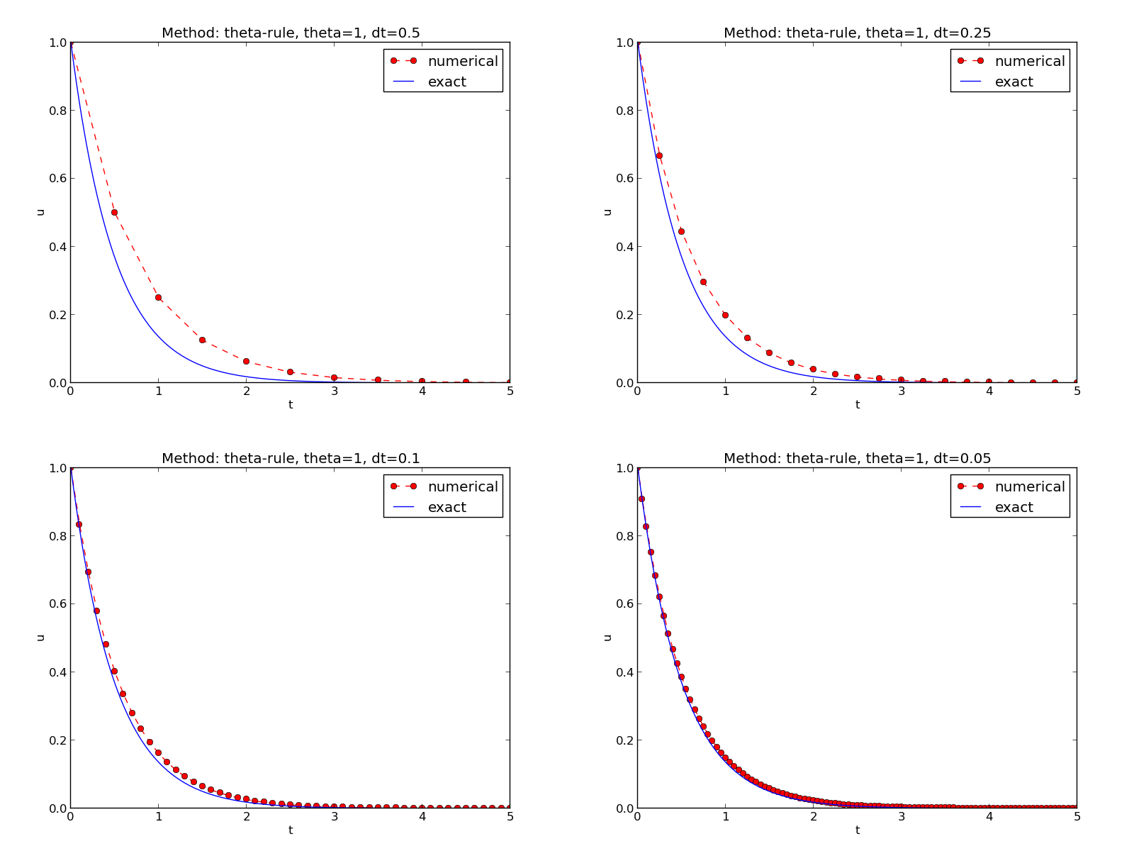
Solution method ($ \theta $-rule): $$ u^{n+1} = \frac{1 - (1-\theta) a\Delta t}{1 + \theta a\Delta t}u^n, \quad u^0=I\tp $$

Plan for the experiments

Plot $ u^n $ against $ \uex = Ie^{-at} $ for various choices of the parameters $ I $, $ a $, $ \Delta t $, and $ \theta $

How does the discrete solution compare with the exact solution when $ \Delta t $ is varied and $ \theta=0,0.5,1 $?

Use the decay_mod.py module (little modification of the plotting, see experiments/decay_mod.py)

Make separate program for running (automating) the experiments (script)

python decay_mod.py --I 1 --a 2 --makeplot --T 5 --dt 0.5 0.25 0.1 0.05

Combine generated figures FE_*.png, BE_*.png, and CN_*.png to new figures with multiple plots

Run script as python decay_exper0.py 0.5 0.25 0.1 0.05 ($ \Delta t $ values on the command line)

Typical plot summarizing the results

Script code

Typical script (small administering program) for running the experiments:

import os, sys

def run_experiments(I=1, a=2, T=5):
    # The command line must contain dt values
    if len(sys.argv) > 1:
        dt_values = [float(arg) for arg in sys.argv[1:]]
    else:
        print 'Usage: %s dt1 dt2 dt3 ...' %  sys.argv[0]
        sys.exit(1)  # abort

    # Run module file as a stand-alone application
    cmd = 'python decay_mod.py --I %g --a %g --makeplot --T %g' % \
          (I, a, T)
    dt_values_str = ' '.join([str(v) for v in dt_values])
    cmd += ' --dt %s' % dt_values_str
    print cmd
    failure = os.system(cmd)
    if failure:
        print 'Command failed:', cmd; sys.exit(1)

    # Combine images into rows with 2 plots in each row
    image_commands = []
    for method in 'BE', 'CN', 'FE':
        pdf_files = ' '.join(['%s_%g.pdf' % (method, dt)
                              for dt in dt_values])
        png_files = ' '.join(['%s_%g.png' % (method, dt)
                              for dt in dt_values])
        image_commands.append(
            'montage -background white -geometry 100%' +
            ' -tile 2x %s %s.png' % (png_files, method))
        image_commands.append(
            'convert -trim %s.png %s.png' % (method, method))
        image_commands.append(
            'convert %s.png -transparent white %s.png' %
            (method, method))
        image_commands.append(
            'pdftk %s output tmp.pdf' % pdf_files)
        num_rows = int(round(len(dt_values)/2.0))
        image_commands.append(
            'pdfnup --nup 2x%d tmp.pdf' % num_rows)
        image_commands.append(
            'pdfcrop tmp-nup.pdf %s.pdf' % method)

    for cmd in image_commands:
        print cmd
        failure = os.system(cmd)
        if failure:
            print 'Command failed:', cmd; sys.exit(1)

    # Remove the files generated above and by decay_mod.py
    from glob import glob
    filenames = glob('*_*.png') + glob('*_*.pdf') + \
                glob('*_*.eps') + glob('tmp*.pdf')
    for filename in filenames:
        os.remove(filename)

if __name__ == '__main__':
    run_experiments()

Complete program: experiments/decay_exper0.py.

Comments to the code

Many useful constructs in the previous script:

[float(arg) for arg in sys.argv[1:]] builds a list of real numbers from all the command-line arguments

failure = os.system(cmd) runs an operating system command (e.g., another program)

sys.exit(1) aborts the program

['%s_%s.png' % (method, dt) for dt in dt_values] builds a list of filenames from a list of numbers (dt_values)

All montage commands for creating composite figures are stored in a list and thereafter executed in a loop

glob.glob('*_*.png') returns a list of the names of all files in the current folder where the filename matches the Unix wildcard notation *_*.png (meaning "any text, underscore, any text, and then `.png`")

os.remove(filename) removes the file with name filename

Interpreting output from other programs

In decay_exper0.py we run a program (os.system) and want to grab the output, e.g.,

Terminal> python decay_plot_mpl.py
0.0   0.40:    2.105E-01
0.0   0.04:    1.449E-02
0.5   0.40:    3.362E-02
0.5   0.04:    1.887E-04
1.0   0.40:    1.030E-01
1.0   0.04:    1.382E-02

Tasks:

read the output from the decay_mod.py program

interpret this output and store the $ E $ values in arrays for each $ \theta $ value

plot $ E $ versus $ \Delta t $, for each $ \theta $, in a log-log plot

Code for grabbing output from another program

Use the subprocess module to grab output:

    from subprocess import Popen, PIPE, STDOUT
    p = Popen(cmd, shell=True, stdout=PIPE, stderr=STDOUT)
    output, dummy = p.communicate()
    failure = p.returncode
    if failure:
        print 'Command failed:', cmd; sys.exit(1)

Code for interpreting the grabbed output

Run through the output string, line by line

If the current line prints $ \theta $, $ \Delta t $, and $ E $, split the line into these three pieces and store the data

Store data in a dictionary errors with keys dt and the three $ \theta $ values

errors = {'dt': dt_values, 1: [], 0: [], 0.5: []}
for line in output.splitlines():
    words = line.split()
    if words[0] in ('0.0', '0.5', '1.0'):  # line with E?
        # typical line: 0.0   1.25:    7.463E+00
        theta = float(words[0])
        E = float(words[2])
        errors[theta].append(E)

Next: plot $ E $ versus $ \Delta t $ for $ \theta=0,0.5,1 $

Complete program: experiments/decay_exper1.py. Fine recipe for

how to run other programs

how to extract and interpret output from other programs

how to automate many manual steps in creating simulations and figures

Making a report

Scientific investigations are best documented in a report!

A sample report

How can we write such a report?

First problem: what format should I write in?

Plain HTML, generated by decay_exper1_html.py

HTML with MathJax, generated by decay_exper1_mathjax.py

LaTeX PDF, based on LaTeX source

Sphinx HTML, based on reStructuredText

Markdown, MediaWiki, ...

DocOnce can generate LaTeX, HTML w/MathJax, Sphinx, Markdown, MediaWiki, ... (DocOnce source for the examples above, and Python program for generating the DocOnce source)

Examples on different report formats

Publishing a complete project

Make folder (directory) tree

Keep track of all files via a version control system (Mercurial, Git, ...)

Publish as private or public repository

Utilize Bitbucket, Googlecode, GitHub, or similar

See the intro to such tools

Study Guide: Scientific software engineering for a simple ODE problem

Sep 25, 2014

Table of contents

Creating user interfaces

Accessing command-line arguments

Reading a sequence of command-line arguments

Implementation

Working with an argument parser

Reading option-values pairs

A graphical user interface

The Parampool package

Making a compute function

The hard part of the compute function: the HTML code

How to embed a PNG plot in HTML code

Generating the user interface

Running the web application

More advanced use

Computing convergence rates

Estimating the convergence rate \( r \)

Implementation

Execution

Debugging via convergence rates

Software engineering

Making a module

Sketch of the module

Test block

Extended test block

Prefixing imported functions by the module name

Downside of module prefix notation

Doctests

Running doctests

Unit testing with nose

Basic use of nose

Example on a nose test in the source code

Example on a nose test in a separate file

The habit of writing nose tests

Purpose of a test function: raise AssertionError if failure

Advantages of nose

Demonstrating nose (ideas)

Demonstrating nose (code)

Floats as test results require careful comparison

Test of wrong use

Test of convergence rates

Classical unit testing with unittest

Basic use of unittest

Demonstration of unittest

Implementing simple problem and solver classes

What to learn

The problem class

Improved problem class

The solver class

The visualizer class

Combing the classes

Implementing more advanced problem and solver classes

A generic class for parameters

The problem class

The solver class

The visualizer class

Performing scientific experiments

Model problem and numerical solution method

Plan for the experiments

Typical plot summarizing the results

Script code

Comments to the code

Interpreting output from other programs

Code for grabbing output from another program

Code for interpreting the grabbed output

Making a report

Publishing a complete project