INF5620 in a nutshell
The new official six-point course description
More specific contents: finite difference methods
More specific contents: finite element methods
More specific contents: nonlinear and advanced problems
Philosophy: simplify, understand, generalize
The exam
Required software
Assumed/ideal background
Start-up example for the course
Start-up example
What to learn in the start-up example; standard topics
What to learn in the start-up example; programming topics
What to learn in the start-up example; mathematical analysis
What to learn in the start-up example; generalizations
Finite difference methods
Topics in the first intro to the finite difference method
A basic model for exponential decay
The ODE model has a range of applications in many fields
The ODE problem has a continuous and discrete version
Continuous problem
Discrete problem
The steps in the finite difference method
Step 1: Discretizing the domain
Step 1: Discretizing the domain
What about a mesh function between the mesh points?
Step 2: Fulfilling the equation at discrete time points
Step 3: Replacing derivatives by finite differences
Step 3: Replacing derivatives by finite differences
Step 4: Formulating a recursive algorithm
Let us apply the scheme by hand
A backward difference
The Backward Euler scheme
A centered difference
The Crank-Nicolson scheme; ideas
The Crank-Nicolson scheme; result
The unifying \( \theta \)-rule
Constant time step
Test the understanding!
Compact operator notation for finite differences
Specific notation for difference operators
The Backward Euler scheme with operator notation
The Forward Euler scheme with operator notation
The Crank-Nicolson scheme with operator notation
Implementation
Requirements of a program
Tools to learn
Why implement in Python?
Why implement in Python?
Algorithm
Translation to Python function
Integer division
Doc strings
Formatting of numbers
Running the program
Plotting the solution
Comparing with the exact solution
Add legends, axes labels, title, and wrap in a function
Plotting with SciTools
Verifying the implementation
Simplest method: run a few algorithmic steps by hand
Comparison with an exact discrete solution
Making a test based on an exact discrete solution
Test the understanding!
Computing the numerical error as a mesh function
Computing the norm of the error
Norms of mesh functions
Implementation of the norm of the error
Comment on array vs scalar computation
Memory-saving implementation
Memory-saving solver function
Reading computed data from file
Usage of memory-saving code
Analysis of finite difference equations
Encouraging numerical solutions
Discouraging numerical solutions; Crank-Nicolson
Discouraging numerical solutions; Forward Euler
Summary of observations
Problem setting
Experimental investigation of oscillatory solutions
Exact numerical solution
Stability
Computation of stability in this problem
Computation of stability in this problem
Explanation of problems with Forward Euler
Explanation of problems with Crank-Nicolson
Summary of stability
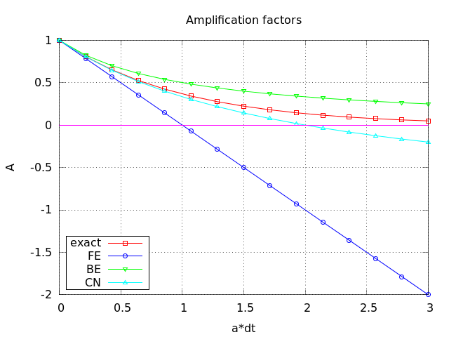
Comparing amplification factors
Plot of amplification factors
Series expansion of amplification factors
Error in amplification factors
The fraction of numerical and exact amplification factors
The true/global error at a point
Computing the global error at a point
Convergence
Integrated errors
Truncation error
Computation of the truncation error
The truncation error for other schemes
Consistency, stability, and convergence
Model extensions
Extension to a variable coefficient; Forward and Backward Euler
Extension to a variable coefficient; Crank-Nicolson
Extension to a variable coefficient; \( \theta \)-rule
Extension to a variable coefficient; operator notation
Extension to a source term
Implementation of the generalized model problem
Implementations of variable coefficients; functions
Implementations of variable coefficients; classes
Implementations of variable coefficients; lambda function
Verification via trivial solutions
Verification via trivial solutions; test function
Verification via manufactured solutions
Linear manufactured solution
Test function for linear manufactured solution
Extension to systems of ODEs
The Backward Euler method gives a system of algebraic equations
Methods for general first-order ODEs
Generic form
The \( \theta \)-rule
Implicit 2-step backward scheme
The Leapfrog scheme
The filtered Leapfrog scheme
2nd-order Runge-Kutta scheme
4th-order Runge-Kutta scheme
2nd-order Adams-Bashforth scheme
3rd-order Adams-Bashforth scheme
The Odespy software
Example: Runge-Kutta methods
Plots from the experiments
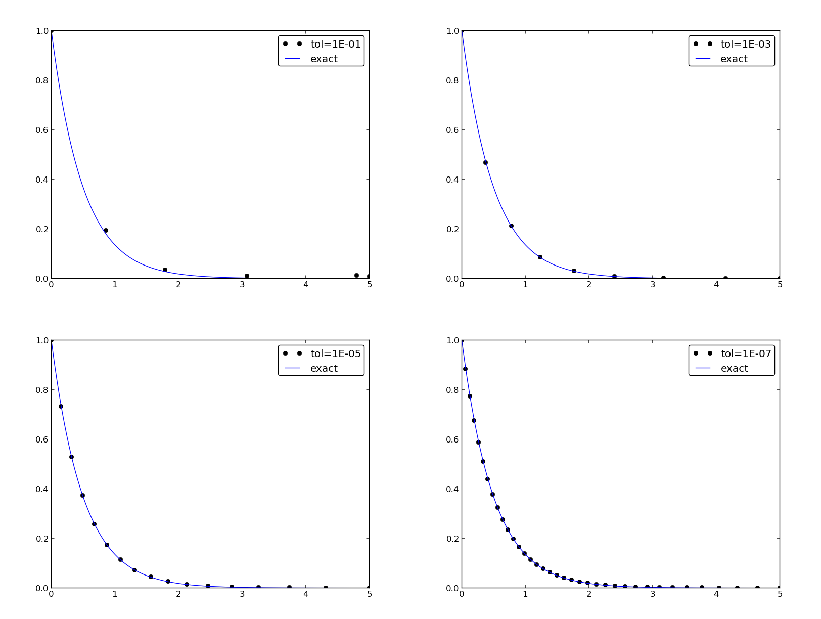
Example: Adaptive Runge-Kutta methods
You see a PDE and can't wait to program a method and visualize a solution! Somebody asks if the solution is right and you can give a convincing answer.
After having completed INF5620 you
numpy, scipy, matplotlib,
sympy, fenics, scitools, ...What if you don't have this ideal background?
$$ u'=-au,\quad u(0)=I,\ t\in (0,T],$$ where \( a>0 \) is a constant.
Everything we do is motivated by what we need as building blocks for solving PDEs!
sympy software
for symbolic computation
The world's simplest (?) ODE: $$ \begin{equation*} u'(t) = -au(t),\quad u(0)=I,\ t\in (0,T] \end{equation*} $$
We can learn a lot about numerical methods, computer implementation, program testing, and real applications of these tools by using this very simple ODE as example. The teaching principle is to keep the math as simple as possible while learning computer tools.
Numerical methods applied to the continuous problem turns it into a discrete problem $$ \begin{equation} u^{n+1} = \mbox{const} u^n, \quad n=0,1,\ldots N_t-1, \quad u^n=I \label{decay:problem:discrete} \end{equation} $$ (varies with discrete mesh points \( t_n \))
Solving a differential equation by a finite difference method consists of four steps:
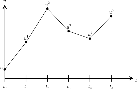
The time domain \( [0,T] \) is represented by a mesh: a finite number of \( N_t+1 \) points $$0 = t_0 < t_1 < t_2 < \cdots < t_{N_t-1} < t_{N_t} = T$$
\( u^n \) is a mesh function, defined at the mesh points \( t_n \), \( n=0,\ldots,N_t \) only.
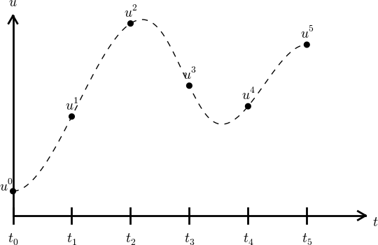
Can extend the mesh function to yield values between mesh points by linear interpolation: $$ \begin{equation} u(t) \approx u^n + \frac{u^{n+1}-u^n}{t_{n+1}-t_n}(t - t_n) \end{equation} $$
Now it is time for the finite difference approximations of derivatives: $$ \begin{equation} u'(t_n) \approx \frac{u^{n+1}-u^{n}}{t_{n+1}-t_n} \label{decay:FEdiff} \end{equation} $$
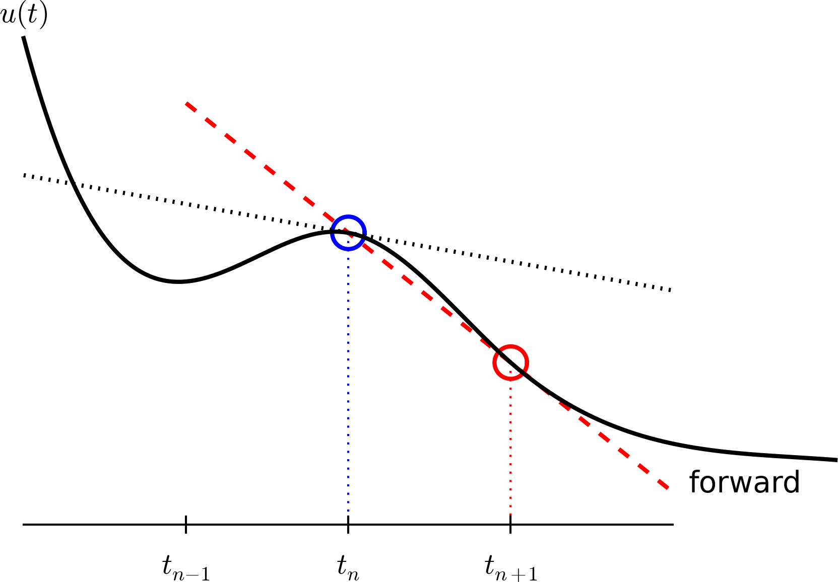
Inserting the finite difference approximation in $$ u'(t_n) = -au(t_n)$$ gives $$ \begin{equation} \frac{u^{n+1}-u^{n}}{t_{n+1}-t_n} = -au^{n},\quad n=0,1,\ldots,N_t-1 \label{decay:step3} \end{equation} $$
(Known as discrete equation, or discrete problem, or finite difference method/scheme)
How can we actually compute the \( u^n \) values?
Solve wrt \( u^{n+1} \) to get the computational formula: $$ \begin{equation} u^{n+1} = u^n - a(t_{n+1} -t_n)u^n \label{decay:FE} \end{equation} $$
Assume constant time spacing: \( \Delta t = t_{n+1}-t_n=\mbox{const} \) $$ \begin{align*} u_0 &= I,\\ u_1 & = u^0 - a\Delta t u^0 = I(1-a\Delta t),\\ u_2 & = I(1-a\Delta t)^2,\\ u^3 &= I(1-a\Delta t)^3,\\ &\vdots\\ u^{N_t} &= I(1-a\Delta t)^{N_t} \end{align*} $$
Ooops - we can find the numerical solution by hand (in this simple example)! No need for a computer (yet)...
Here is another finite difference approximation to the derivative (backward difference): $$ \begin{equation} u'(t_n) \approx \frac{u^{n}-u^{n-1}}{t_{n}-t_{n-1}} \label{decay:BEdiff} \end{equation} $$
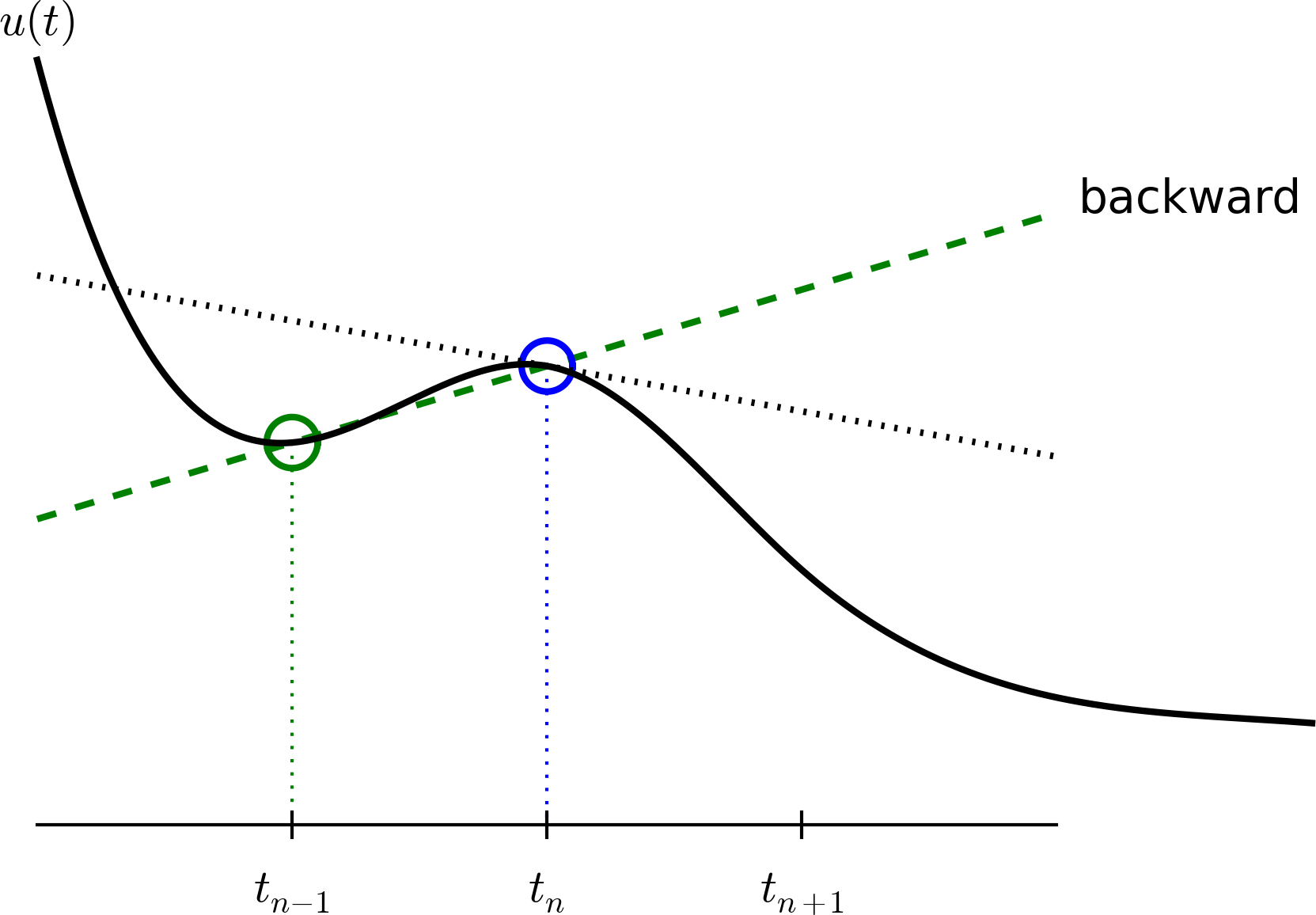
Inserting the finite difference approximation in \( u'(t_n)=-au(t_n) \) yields the Backward Euler (BE) scheme: $$ \begin{equation} \frac{u^{n}-u^{n-1}}{t_{n}-t_{n-1}} = -a u^n \label{decay:BE0} \end{equation} $$ Solve with respect to the unknown \( u^{n+1} \): $$ \begin{equation} u^{n+1} = \frac{1}{1+ a(t_{n+1}-t_n)} u^n \label{decay:BE} \end{equation} $$
Centered differences are better approximations than forward or backward differences.
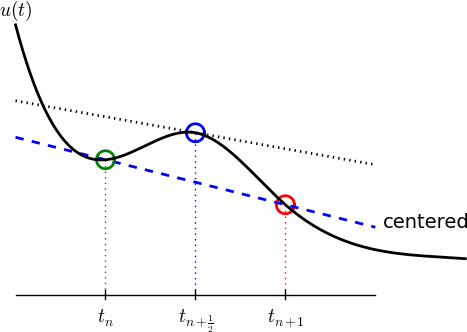
Idea 1: let the ODE hold at \( t_{n+\half} \) $$ u'(t_{n+\half}) = -au(t_{n+\half})$$
Idea 2: approximate \( u'(t_{n+\half} \) by a centered difference $$ \begin{equation} u'(t_{n+\half}) \approx \frac{u^{n+1}-u^n}{t_{n+1}-t_n} \label{decay:CNdiff} \end{equation} $$
Problem: \( u(t_{n+\half}) \) is not defined, only \( u^n=u(t_n) \) and \( u^{n+1}=u(t_{n+1}) \)
Solution: $$ u(t_{n+\half}) \approx \half(u^n + u^{n+1}) $$
Result: $$ \begin{equation} \frac{u^{n+1}-u^n}{t_{n+1}-t_n} = -a\half (u^n + u^{n+1}) \label{decay:CN1} \end{equation} $$
Solve wrt to \( u^{n+1} \): $$ \begin{equation} u^{n+1} = \frac{1-\half a(t_{n+1}-t_n)}{1 + \half a(t_{n+1}-t_n)}u^n \label{decay:CN} \end{equation} $$ This is a Crank-Nicolson (CN) scheme or a midpoint or centered scheme.
The Forward Euler, Backward Euler, and Crank-Nicolson schemes can be formulated as one scheme with a varying parameter \( \theta \): $$ \begin{equation} \frac{u^{n+1}-u^{n}}{t_{n+1}-t_n} = -a (\theta u^{n+1} + (1-\theta) u^{n}) \label{decay:th0} \end{equation} $$
Very common assumption (not important, but exclusively used for simplicity hereafter): constant time step \( t_{n+1}-t_n\equiv\Delta t \)
$$ \begin{align} u^{n+1} &= (1 - a\Delta t )u^n \quad (\hbox{FE}) \label{decay:FE:u}\\ u^{n+1} &= \frac{1}{1+ a\Delta t} u^n \quad (\hbox{BE}) \label{decay:BE:u}\\ u^{n+1} &= \frac{1-\half a\Delta t}{1 + \half a\Delta t} u^n \quad (\hbox{CN}) \label{decay:CN:u}\\ u^{n+1} &= \frac{1 - (1-\theta) a\Delta t}{1 + \theta a\Delta t}u^n \quad (\theta-\hbox{rule}) \label{decay:th:u} \end{align} $$
Derive Forward Euler, Backward Euler, and Crank-Nicolson schemes for Newton's law of cooling: $$ T' = -k(T-T_s),\quad T(0)=T_0,\ t\in (0,t_{\mbox{end}}]$$
Physical quantities:
Forward difference: $$ \begin{equation} [D_t^+u]^n = \frac{u^{n+1} - u^{n}}{\Delta t} \approx \frac{d}{dt} u(t_n) \label{fd:D:f} \end{equation} $$ Centered difference: $$ \begin{equation} [D_tu]^n = \frac{u^{n+\half} - u^{n-\half}}{\Delta t} \approx \frac{d}{dt} u(t_n), \label{fd:D:c} \end{equation} $$
Backward difference: $$ \begin{equation} [D_t^-u]^n = \frac{u^{n} - u^{n-1}}{\Delta t} \approx \frac{d}{dt} u(t_n) \label{fd:D:b} \end{equation} $$
Common to put the whole equation inside square brackets: $$ \begin{equation} [D_t^- u = -au]^n \end{equation} $$
Introduce an averaging operator: $$ \begin{equation} [\overline{u}^{t}]^n = \half (u^{n-\half} + u^{n+\half} ) \approx u(t_n) \label{fd:mean:a} \end{equation} $$
The Crank-Nicolson scheme can then be written as $$ \begin{equation} [D_t u = -a\overline{u}^t]^{n+\half} \label{fd:compact:ex:CN} \end{equation} $$
Test: use the definitions and write out the above formula to see that it really is the Crank-Nicolson scheme!
Model: $$ u'(t) = -au(t),\quad t\in (0,T], \quad u(0)=I $$
Numerical method: $$ u^{n+1} = \frac{1 - (1-\theta) a\Delta t}{1 + \theta a\Delta t}u^n $$ for \( \theta\in [0,1] \). Note
All programs are in the directory src/decay.
u.
1 2 3 4 5 6 7 8 9 10 11 12 13 | from numpy import *
def solver(I, a, T, dt, theta):
"""Solve u'=-a*u, u(0)=I, for t in (0,T] with steps of dt."""
Nt = int(T/dt) # no of time intervals
T = Nt*dt # adjust T to fit time step dt
u = zeros(Nt+1) # array of u[n] values
t = linspace(0, T, Nt+1) # time mesh
u[0] = I # assign initial condition
for n in range(0, Nt): # n=0,1,...,Nt-1
u[n+1] = (1 - (1-theta)*a*dt)/(1 + theta*dt*a)*u[n]
return u, t
|
Note about the for loop: range(0, Nt, s) generates all integers
from 0 to Nt in steps of s (default 1), but not including Nt (!).
Sample call:
1 | u, t = solver(I=1, a=2, T=8, dt=0.8, theta=1)
|
Python applies integer division: 1/2 is 0, while 1./2 or 1.0/2 or
1/2. or 1/2.0 or 1.0/2.0 all give 0.5.
A safer solver function (dt = float(dt) - guarantee float):
1 2 3 4 5 6 7 8 9 10 11 12 13 14 | from numpy import *
def solver(I, a, T, dt, theta):
"""Solve u'=-a*u, u(0)=I, for t in (0,T] with steps of dt."""
dt = float(dt) # avoid integer division
Nt = int(round(T/dt)) # no of time intervals
T = Nt*dt # adjust T to fit time step dt
u = zeros(Nt+1) # array of u[n] values
t = linspace(0, T, Nt+1) # time mesh
u[0] = I # assign initial condition
for n in range(0, Nt): # n=0,1,...,Nt-1
u[n+1] = (1 - (1-theta)*a*dt)/(1 + theta*dt*a)*u[n]
return u, t
|
1 2 3 4 5 6 7 8 9 10 11 12 13 14 15 | def solver(I, a, T, dt, theta):
"""
Solve
u'(t) = -a*u(t),
with initial condition u(0)=I, for t in the time interval
(0,T]. The time interval is divided into time steps of
length dt.
theta=1 corresponds to the Backward Euler scheme, theta=0
to the Forward Euler scheme, and theta=0.5 to the Crank-
Nicolson method.
"""
...
|
Can control formatting of reals and integers through the printf format:
1 | print 't=%6.3f u=%g' % (t[i], u[i])
|
Or the alternative format string syntax:
1 | print 't={t:6.3f} u={u:g}'.format(t=t[i], u=u[i])
|
How to run the program decay_v1.py:
1 | Terminal> python decay_v1.py
|
Can also run it as "normal" Unix programs: ./decay_v1.py if the
first line is
1 | `#!/usr/bin/env python`
|
Then
1 2 | Terminal> chmod a+rx decay_v1.py
Terminal> ./decay_v1.py
|
Basic syntax:
1 2 3 4 | from matplotlib.pyplot import *
plot(t, u)
show()
|
Can (and should!) add labels on axes, title, legends.
Python function for the exact solution \( \uex(t)=Ie^{-at} \):
1 2 | def exact_solution(t, I, a):
return I*exp(-a*t)
|
Quick plotting:
1 2 | u_e = exact_solution(t, I, a)
plot(t, u, t, u_e)
|
Problem: \( \uex(t) \) applies the same mesh as \( u^n \) and looks as a piecewise linear function.
Remedy: Introduce a very fine mesh for \( \uex \).
1 2 3 4 5 | t_e = linspace(0, T, 1001) # fine mesh
u_e = exact_solution(t_e, I, a)
plot(t_e, u_e, 'b-', # blue line for u_e
t, u, 'r--o') # red dashes w/circles
|
1 2 3 4 5 6 7 8 9 10 11 12 13 14 15 16 | from matplotlib.pyplot import *
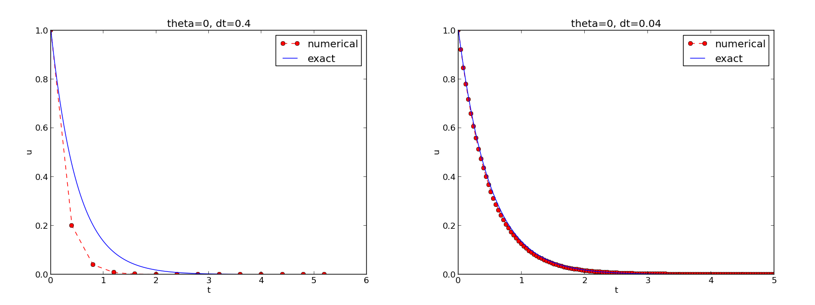
def plot_numerical_and_exact(theta, I, a, T, dt):
"""Compare the numerical and exact solution in a plot."""
u, t = solver(I=I, a=a, T=T, dt=dt, theta=theta)
t_e = linspace(0, T, 1001) # fine mesh for u_e
u_e = exact_solution(t_e, I, a)
plot(t, u, 'r--o', # red dashes w/circles
t_e, u_e, 'b-') # blue line for exact sol.
legend(['numerical', 'exact'])
xlabel('t')
ylabel('u')
title('theta=%g, dt=%g' % (theta, dt))
savefig('plot_%s_%g.png' % (theta, dt))
|
Complete code in decay_v2.py
SciTools provides a unified plotting interface (Easyviz) to many different plotting packages: Matplotlib, Gnuplot, Grace, VTK, OpenDX, ...
Can use Matplotlib (MATLAB-like) syntax,
or a more compact plot function syntax:
1 2 3 4 5 6 7 8 9 10 | from scitools.std import *
plot(t, u, 'r--o', # red dashes w/circles
t_e, u_e, 'b-', # blue line for exact sol.
legend=['numerical', 'exact'],
xlabel='t',
ylabel='u',
title='theta=%g, dt=%g' % (theta, dt),
savefig='%s_%g.png' % (theta2name[theta], dt),
show=True)
|
Change backend (plotting engine, Matplotlib by default):
1 2 | Terminal> python decay_plot_st.py --SCITOOLS_easyviz_backend gnuplot
Terminal> python decay_plot_st.py --SCITOOLS_easyviz_backend grace
|
Use a calculator (\( I=0.1 \), \( \theta=0.8 \), \( \Delta t =0.8 \)): $$ A\equiv \frac{1 - (1-\theta) a\Delta t}{1 + \theta a \Delta t} = 0.298245614035$$ $$ \begin{align*} u^1 &= AI=0.0298245614035,\\ u^2 &= Au^1= 0.00889504462912,\\ u^3 &=Au^2= 0.00265290804728 \end{align*} $$
See the function verify_three_steps in decay_verf1.py.
Compare computed numerical solution with a closed-form exact discrete solution (if possible).
Define $$ A = \frac{1 - (1-\theta) a\Delta t}{1 + \theta a \Delta t}$$ Repeated use of the \( \theta \)-rule: $$ \begin{align*} u^0 &= I,\\ u^1 &= Au^0 = AI\\ u^n &= A^nu^{n-1} = A^nI \end{align*} $$
The exact discrete solution is $$ \begin{equation} u^n = IA^n \label{decay:un:exact} \end{equation} $$
Understand what \( n \) in \( u^n \) and in \( A^n \) means!
Test if $$ \max_n |u^n - \uex(t_n)| < \epsilon\sim 10^{-15}$$
Implementation in decay_verf2.py.
Make a program for solving Newton's law of cooling $$ T' = -k(T-T_s),\quad T(0)=T_0,\ t\in (0,t_{\mbox{end}}]$$ with the Forward Euler, Backward Euler, and Crank-Nicolson schemes (or a \( \theta \) scheme). Verify the implementation.
Task: compute the numerical error \( e^n = \uex(t_n) - u^n \)
Exact solution: \( \uex(t)=Ie^{-at} \), implemented as
1 2 | def exact_solution(t, I, a):
return I*exp(-a*t)
|
Compute \( e^n \) by
1 2 3 | u, t = solver(I, a, T, dt, theta) # Numerical solution
u_e = exact_solution(t, I, a)
e = u_e - u
|
exact_solution(t, I, a) works with t as arrayexp from numpy (not math)e = u_e - u: array subtraction
Common simplification yields the \( L^2 \) norm of a mesh function: $$ ||f^n||_{\ell^2} = \left(\Delta t\sum_{n=0}^{N_t} (f^n)^2\right)^{1/2}$$
Python w/array arithmetics:
1 2 | e = exact_solution(t) - u
E = sqrt(dt*sum(e**2))
|
Scalar computing of E = sqrt(dt*sum(e**2)):
1 2 3 4 5 6 7 8 9 10 11 12 13 | m = len(u) # length of u array (alt: u.size)
u_e = zeros(m)
t = 0
for i in range(m):
u_e[i] = exact_solution(t, a, I)
t = t + dt
e = zeros(m)
for i in range(m):
e[i] = u_e[i] - u[i]
s = 0 # summation variable
for i in range(m):
s = s + e[i]**2
error = sqrt(dt*s)
|
Obviously, scalar computing
Compute on entire arrays (when possible)!
u, i.e., \( u^n \) for \( n=0,1,\ldots,N_t \)u, \( u^n \) in u_1 (float)u in a file, read file later for plotting
1 2 3 4 5 6 7 8 9 10 11 12 13 14 15 16 17 18 19 20 21 | def solver_memsave(I, a, T, dt, theta, filename='sol.dat'):
"""
Solve u'=-a*u, u(0)=I, for t in (0,T] with steps of dt.
Minimum use of memory. The solution is stored in a file
(with name filename) for later plotting.
"""
dt = float(dt) # avoid integer division
Nt = int(round(T/dt)) # no of intervals
outfile = open(filename, 'w')
# u: time level n+1, u_1: time level n
t = 0
u_1 = I
outfile.write('%.16E %.16E\n' % (t, u_1))
for n in range(1, Nt+1):
u = (1 - (1-theta)*a*dt)/(1 + theta*dt*a)*u_1
u_1 = u
t += dt
outfile.write('%.16E %.16E\n' % (t, u))
outfile.close()
return u, t
|
1 2 3 4 5 6 7 8 9 10 11 | def read_file(filename='sol.dat'):
infile = open(filename, 'r')
u = []; t = []
for line in infile:
words = line.split()
if len(words) != 2:
print 'Found more than two numbers on a line!', words
sys.exit(1) # abort
t.append(float(words[0]))
u.append(float(words[1]))
return np.array(t), np.array(u)
|
Simpler code with numpy functionality for reading/writing tabular data:
1 2 3 4 5 | def read_file_numpy(filename='sol.dat'):
data = np.loadtxt(filename)
t = data[:,0]
u = data[:,1]
return t, u
|
Similar function np.savetxt, but then we need all \( u^n \) and \( t^n \) values
in a two-dimensional array (which we try to prevent now!).
1 2 3 4 5 6 7 8 9 10 11 | def explore(I, a, T, dt, theta=0.5, makeplot=True):
filename = 'u.dat'
u, t = solver_memsave(I, a, T, dt, theta, filename)
t, u = read_file(filename)
u_e = exact_solution(t, I, a)
e = u_e - u
E = np.sqrt(dt*np.sum(e**2))
if makeplot:
plt.figure()
...
|
Complete program: decay_memsave.py.
Model: $$ \begin{equation} u'(t) = -au(t),\quad u(0)=I \end{equation} $$
Method: $$ \begin{equation} u^{n+1} = \frac{1 - (1-\theta) a\Delta t}{1 + \theta a\Delta t}u^n \label{decay:analysis:scheme} \end{equation} $$
How good is this method? Is it safe to use it?
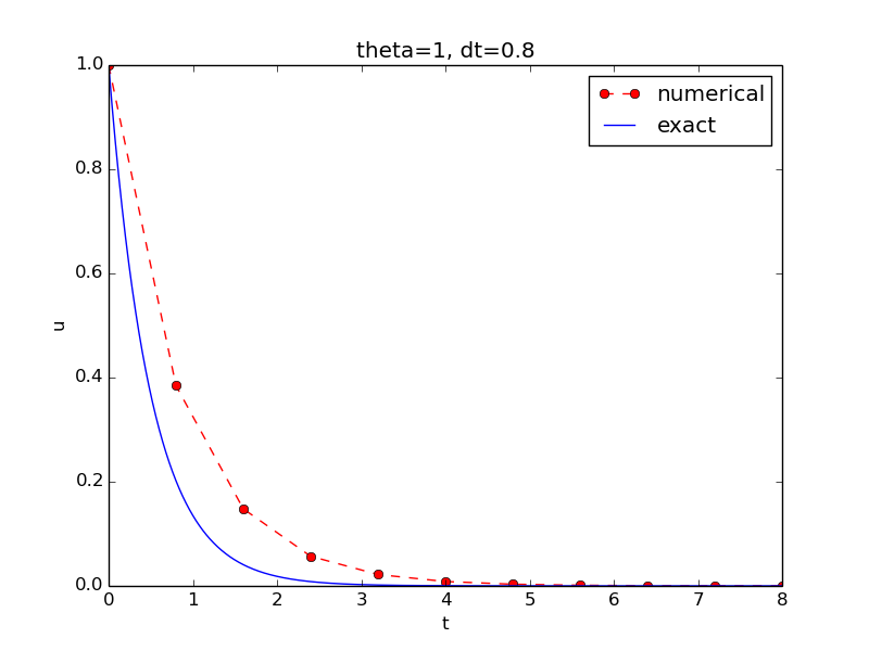
\( I=1 \), \( a=2 \), \( \theta =1,0.5, 0 \), \( \Delta t=1.25, 0.75, 0.5, 0.1 \).
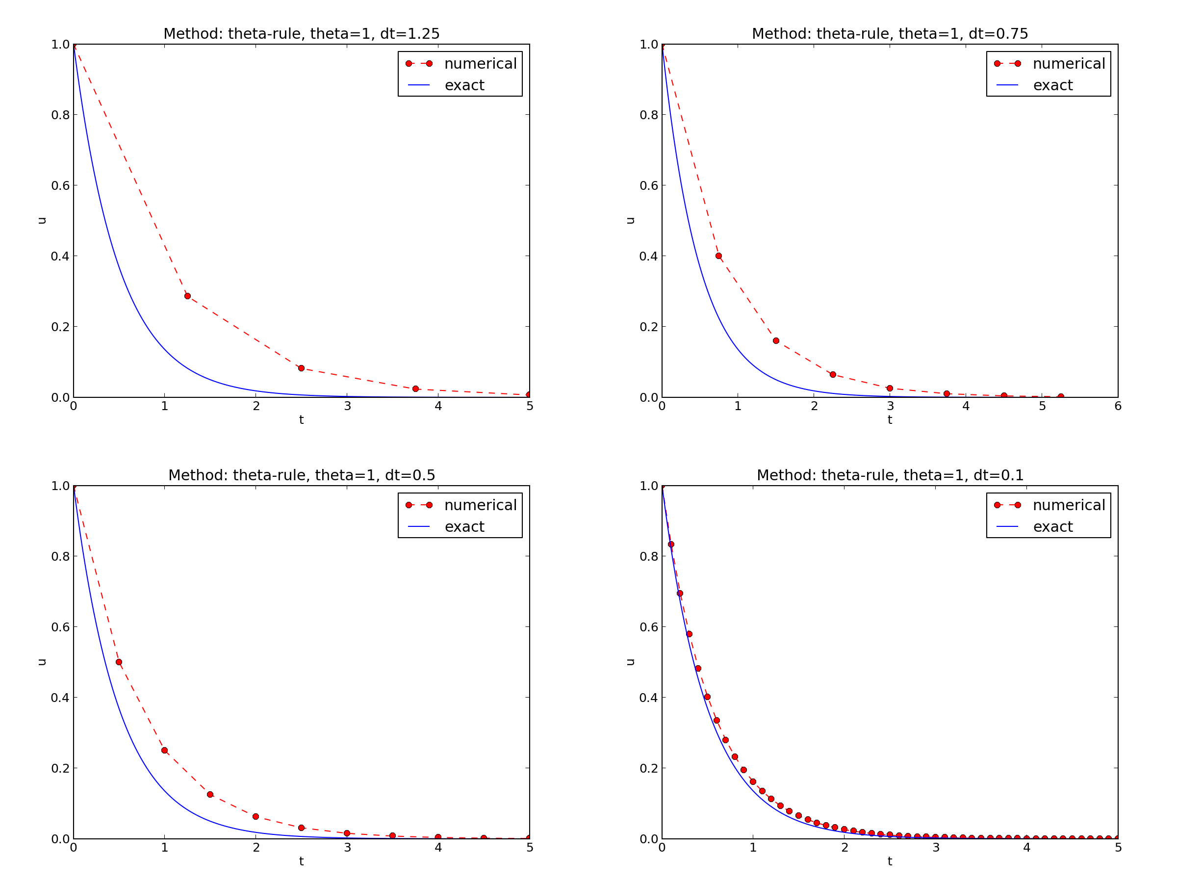
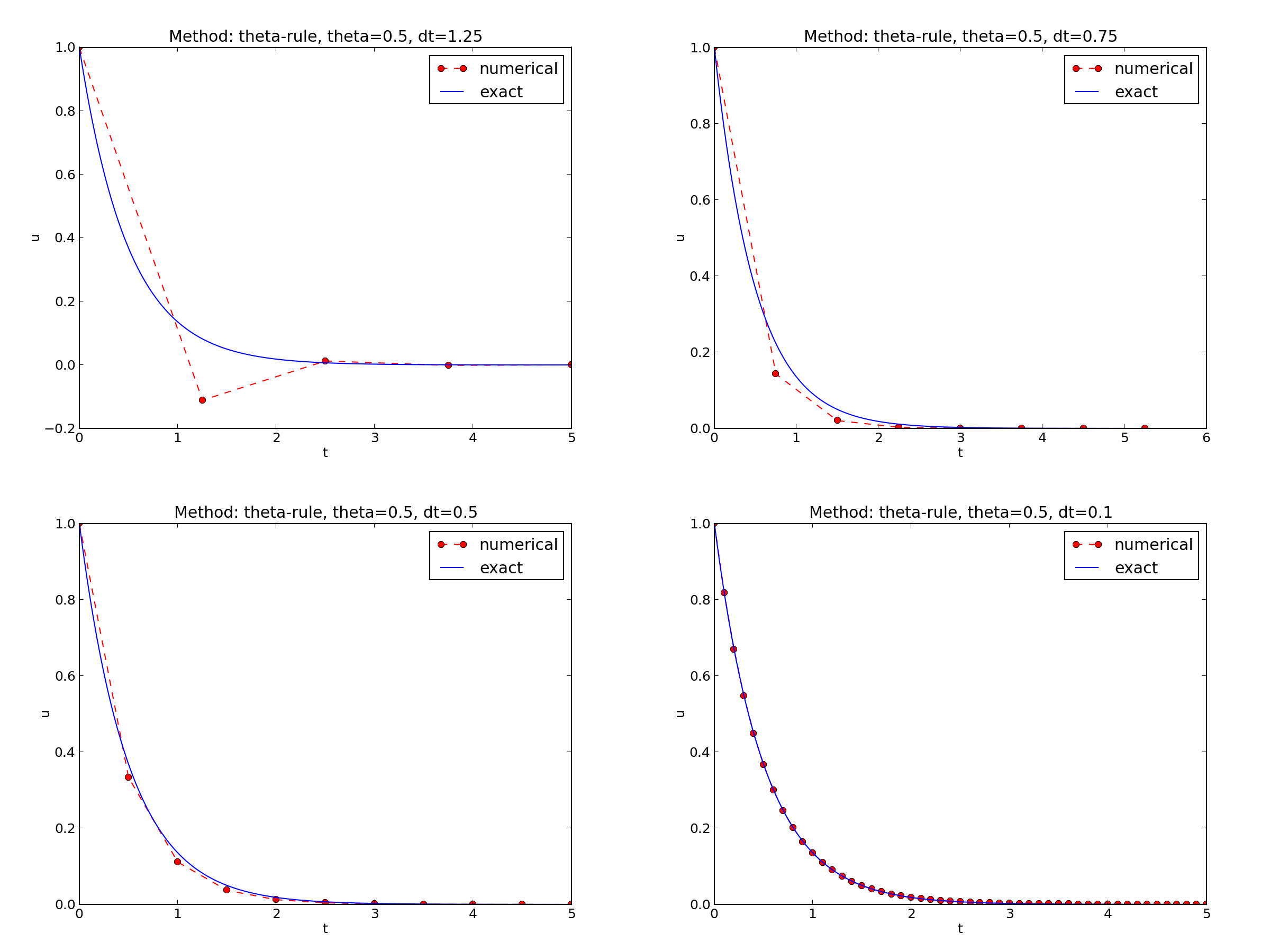
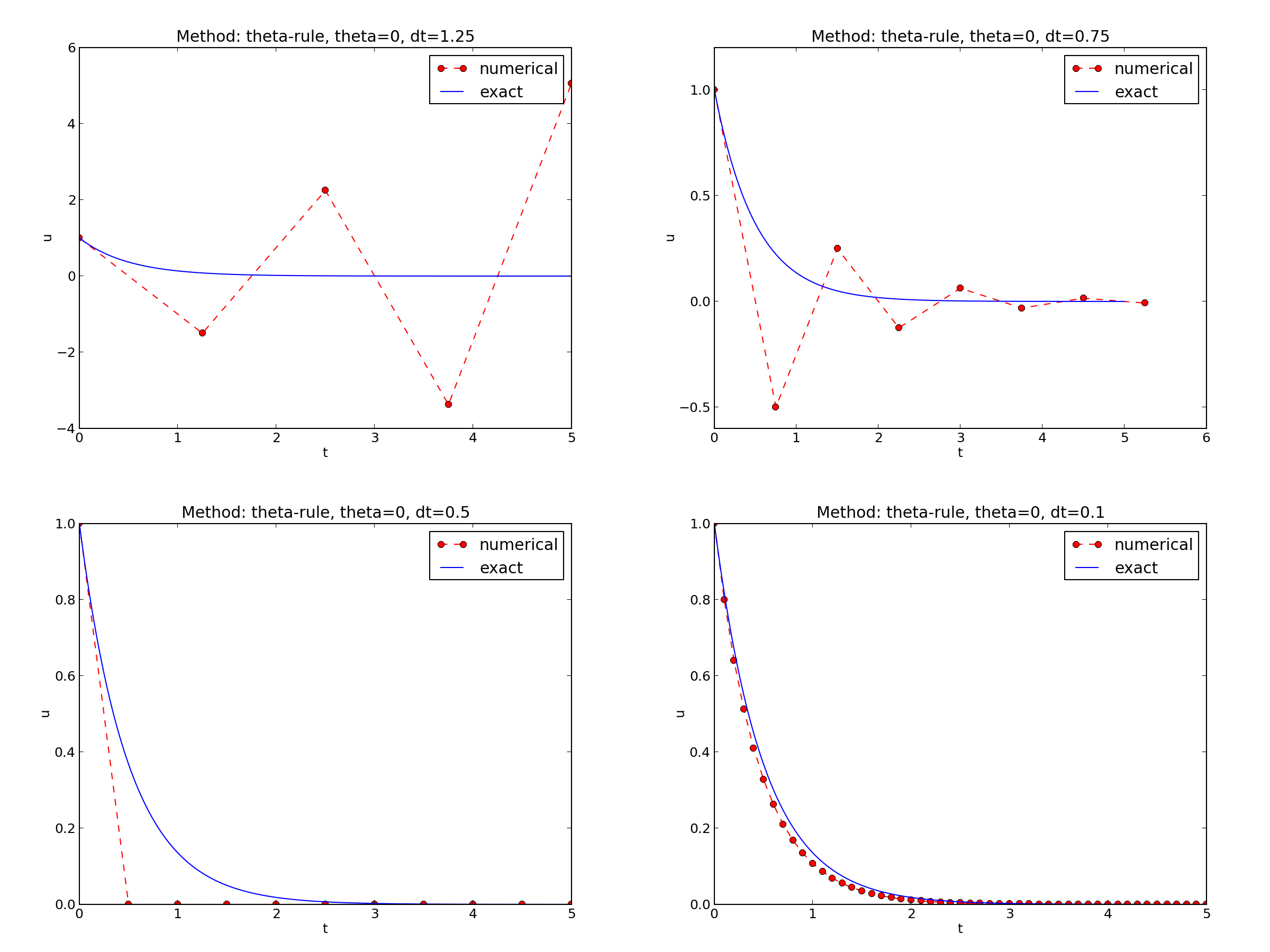
The characteristics of the displayed curves can be summarized as follows:
We ask the question
The solution is oscillatory if $$ u^{n} > u^{n-1}$$
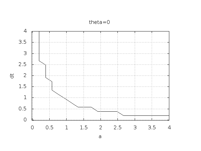
Seems that \( a\Delta t < 1 \) for FE and 2 for CN.
Starting with \( u^0=I \), the simple recursion \eqref{decay:analysis:scheme} can be applied repeatedly \( n \) times, with the result that $$ \begin{equation} u^{n} = IA^n,\quad A = \frac{1 - (1-\theta) a\Delta t}{1 + \theta a\Delta t} \label{decay:analysis:unex} \end{equation} $$
Such an exact discrete solution is unusual, but very handy for analysis.
Since \( u^n\sim A^n \),
\( A < 0 \) if $$ \frac{1 - (1-\theta) a\Delta t}{1 + \theta a\Delta t} < 0 $$ To avoid oscillatory solutions we must have \( A> 0 \) and $$ \begin{equation} \Delta t < \frac{1}{(1-\theta)a}\ \end{equation} $$
\( |A|\leq 1 \) means \( -1\leq A\leq 1 \) $$ \begin{equation} -1\leq\frac{1 - (1-\theta) a\Delta t}{1 + \theta a\Delta t} \leq 1 \label{decay:th:stability} \end{equation} $$ \( -1 \) is the critical limit: $$ \begin{align*} \Delta t &\leq \frac{2}{(1-2\theta)a},\quad \theta < \half\\ \Delta t &\geq \frac{2}{(1-2\theta)a},\quad \theta > {\half} \end{align*} $$
\( u^{n+1} \) is an amplification \( A \) of \( u^n \): $$ u^{n+1} = Au^n,\quad A = \frac{1 - (1-\theta) a\Delta t}{1 + \theta a\Delta t} $$
The exact solution is also an amplification: $$ u(t_{n+1}) = \Aex u(t_n), \quad \Aex = e^{-a\Delta t}$$
A possible measure of accuracy: \( \Aex - A \)
To investigate \( \Aex - A \) mathematically, we can Taylor expand the expression, using \( p=a\Delta t \) as variable.
1 2 3 4 5 6 7 8 9 10 11 12 13 14 15 16 17 18 19 20 21 22 | >>> from sympy import *
>>> # Create p as a mathematical symbol with name 'p'
>>> p = Symbol('p')
>>> # Create a mathematical expression with p
>>> A_e = exp(-p)
>>>
>>> # Find the first 6 terms of the Taylor series of A_e
>>> A_e.series(p, 0, 6)
1 + (1/2)*p**2 - p - 1/6*p**3 - 1/120*p**5 + (1/24)*p**4 + O(p**6)
>>> theta = Symbol('theta')
>>> A = (1-(1-theta)*p)/(1+theta*p)
>>> FE = A_e.series(p, 0, 4) - A.subs(theta, 0).series(p, 0, 4)
>>> BE = A_e.series(p, 0, 4) - A.subs(theta, 1).series(p, 0, 4)
>>> half = Rational(1,2) # exact fraction 1/2
>>> CN = A_e.series(p, 0, 4) - A.subs(theta, half).series(p, 0, 4)
>>> FE
(1/2)*p**2 - 1/6*p**3 + O(p**4)
>>> BE
-1/2*p**2 + (5/6)*p**3 + O(p**4)
>>> CN
(1/12)*p**3 + O(p**4)
|
Focus: the error measure \( A-\Aex \) as function of \( \Delta t \) (recall that \( p=a\Delta t \)): $$ \begin{equation} A-\Aex = \left\lbrace\begin{array}{ll} \Oof{\Delta t^2}, & \hbox{Forward and Backward Euler},\\ \Oof{\Delta t^3}, & \hbox{Crank-Nicolson} \end{array}\right. \end{equation} $$
Focus: the error measure \( 1-A/\Aex \) as function of \( p=a\Delta t \):
1 2 3 4 5 6 7 8 9 | >>> FE = 1 - (A.subs(theta, 0)/A_e).series(p, 0, 4)
>>> BE = 1 - (A.subs(theta, 1)/A_e).series(p, 0, 4)
>>> CN = 1 - (A.subs(theta, half)/A_e).series(p, 0, 4)
>>> FE
(1/2)*p**2 + (1/3)*p**3 + O(p**4)
>>> BE
-1/2*p**2 + (1/3)*p**3 + O(p**4)
>>> CN
(1/12)*p**3 + O(p**4)
|
Same leading-order terms as for the error measure \( A-\Aex \).
1 2 3 4 5 6 7 8 9 10 11 12 | >>> n = Symbol('n')
>>> u_e = exp(-p*n) # I=1
>>> u_n = A**n # I=1
>>> FE = u_e.series(p, 0, 4) - u_n.subs(theta, 0).series(p, 0, 4)
>>> BE = u_e.series(p, 0, 4) - u_n.subs(theta, 1).series(p, 0, 4)
>>> CN = u_e.series(p, 0, 4) - u_n.subs(theta, half).series(p, 0, 4)
>>> FE
(1/2)*n*p**2 - 1/2*n**2*p**3 + (1/3)*n*p**3 + O(p**4)
>>> BE
(1/2)*n**2*p**3 - 1/2*n*p**2 + (1/3)*n*p**3 + O(p**4)
>>> CN
(1/12)*n*p**3 + O(p**4)
|
Substitute \( n \) by \( t/\Delta t \):
The numerical scheme is convergent if the global error \( e^n\rightarrow 0 \) as \( \Delta t\rightarrow 0 \). If the error has a leading order term \( \Delta t^r \), the convergence rate is of order \( r \).
Focus: norm of the numerical error $$ ||e^n||_{\ell^2} = \sqrt{\Delta t\sum_{n=0}^{N_t} ({\uex}(t_n) - u^n)^2}$$
Forward and Backward Euler: $$ ||e^n||_{\ell^2} = \frac{1}{4}\sqrt{\frac{T^3}{3}} a^2\Delta t$$
Crank-Nicolson: $$ ||e^n||_{\ell^2} = \frac{1}{12}\sqrt{\frac{T^3}{3}}a^3\Delta t^2$$
Analysis of both the pointwise and the time-integrated true errors:
Backward Euler: $$ R^n \approx -\half\uex''(t_n)\Delta t $$
Crank-Nicolson: $$ R^{n+\half} \approx \frac{1}{24}\uex'''(t_{n+\half})\Delta t^2$$
(Consistency and stability is in most problems much easier to establish than convergence.)
The Forward Euler scheme: $$ \begin{equation} \frac{u^{n+1} - u^n}{\Delta t} = -a(t_n)u^n \end{equation} $$
The Backward Euler scheme: $$ \begin{equation} \frac{u^{n} - u^{n-1}}{\Delta t} = -a(t_n)u^n \end{equation} $$
Eevaluting \( a(t_{n+\half}) \) and using an average for \( u \): $$ \begin{equation} \frac{u^{n+1} - u^{n}}{\Delta t} = -a(t_{n+\half})\half(u^n + u^{n+1}) \end{equation} $$
Using an average for \( a \) and \( u \): $$ \begin{equation} \frac{u^{n+1} - u^{n}}{\Delta t} = -\half(a(t_n)u^n + a(t_{n+1})u^{n+1}) \end{equation} $$
The \( \theta \)-rule unifies the three mentioned schemes, $$ \begin{equation} \frac{u^{n+1} - u^{n}}{\Delta t} = -a((1-\theta)t_n + \theta t_{n+1})((1-\theta) u^n + \theta u^{n+1}) \end{equation} $$ or, $$ \begin{equation} \frac{u^{n+1} - u^{n}}{\Delta t} = -(1-\theta) a(t_n)u^n - \theta a(t_{n+1})u^{n+1} \end{equation} $$
Implementation where \( a(t) \) and \( b(t) \) are given as Python functions (see file decay_vc.py):
1 2 3 4 5 6 7 8 9 10 11 12 13 14 15 16 17 18 | def solver(I, a, b, T, dt, theta):
"""
Solve u'=-a(t)*u + b(t), u(0)=I,
for t in (0,T] with steps of dt.
a and b are Python functions of t.
"""
dt = float(dt) # avoid integer division
Nt = int(round(T/dt)) # no of time intervals
T = Nt*dt # adjust T to fit time step dt
u = zeros(Nt+1) # array of u[n] values
t = linspace(0, T, Nt+1) # time mesh
u[0] = I # assign initial condition
for n in range(0, Nt): # n=0,1,...,Nt-1
u[n+1] = ((1 - dt*(1-theta)*a(t[n]))*u[n] + \
dt*(theta*b(t[n+1]) + (1-theta)*b(t[n])))/\
(1 + dt*theta*a(t[n+1]))
return u, t
|
Plain functions:
1 2 3 4 5 | def a(t):
return a_0 if t < tp else k*a_0
def b(t):
return 1
|
Better implementation: class with the parameters a0, tp, and k
as attributes and a special method __call__ for evaluating \( a(t) \):
1 2 3 4 5 6 7 8 | class A:
def __init__(self, a0=1, k=2):
self.a0, self.k = a0, k
def __call__(self, t):
return self.a0 if t < self.tp else self.k*self.a0
a = A(a0=2, k=1) # a behaves as a function a(t)
|
Quick writing: a one-liner lambda function
1 | a = lambda t: a_0 if t < tp else k*a_0
|
In general,
1 | f = lambda arg1, arg2, ...: expressin
|
is equivalent to
1 2 | def f(arg1, arg2, ...):
return expression
|
One can use lambda functions directly in calls:
1 | u, t = solver(1, lambda t: 1, lambda t: 1, T, dt, theta)
|
for a problem \( u'=-u+1 \), \( u(0)=1 \).
A lambda function can appear anywhere where a variable can appear.
1 2 3 4 5 6 7 8 9 10 11 12 13 14 15 16 17 18 19 20 21 22 23 | def test_constant_solution():
"""
Test problem where u=u_const is the exact solution, to be
reproduced (to machine precision) by any relevant method.
"""
def exact_solution(t):
return u_const
def a(t):
return 2.5*(1+t**3) # can be arbitrary
def b(t):
return a(t)*u_const
u_const = 2.15
theta = 0.4; I = u_const; dt = 4
Nt = 4 # enough with a few steps
u, t = solver(I=I, a=a, b=b, T=Nt*dt, dt=dt, theta=theta)
print u
u_e = exact_solution(t)
difference = abs(u_e - u).max() # max deviation
tol = 1E-14
assert difference < tol
|
\( u^n = ct_n+I \) fulfills the discrete equations!
First, $$ \begin{align} \lbrack D_t^+ t\rbrack^n &= \frac{t_{n+1}-t_n}{\Delta t}=1, \label{decay:fd2:Dop:tn:fw}\\ \lbrack D_t^- t\rbrack^n &= \frac{t_{n}-t_{n-1}}{\Delta t}=1, \label{decay:fd2:Dop:tn:bw}\\ \lbrack D_t t\rbrack^n &= \frac{t_{n+\half}-t_{n-\half}}{\Delta t}=\frac{(n+\half)\Delta t - (n-\half)\Delta t}{\Delta t}=1\label{decay:fd2:Dop:tn:cn} \end{align} $$
Forward Euler: $$ [D^+ u = -au + b]^n $$
\( a^n=a(t_n) \), \( b^n=c + a(t_n)(ct_n + I) \), and \( u^n=ct_n + I \) results in $$ c = -a(t_n)(ct_n+I) + c + a(t_n)(ct_n + I) = c $$
1 2 3 4 5 6 7 8 9 10 11 12 13 14 15 16 17 18 19 20 21 22 23 | def test_linear_solution():
"""
Test problem where u=c*t+I is the exact solution, to be
reproduced (to machine precision) by any relevant method.
"""
def exact_solution(t):
return c*t + I
def a(t):
return t**0.5 # can be arbitrary
def b(t):
return c + a(t)*exact_solution(t)
theta = 0.4; I = 0.1; dt = 0.1; c = -0.5
T = 4
Nt = int(T/dt) # no of steps
u, t = solver(I=I, a=a, b=b, T=Nt*dt, dt=dt, theta=theta)
u_e = exact_solution(t)
difference = abs(u_e - u).max() # max deviation
print difference
tol = 1E-14 # depends on c!
assert difference < tol
|
Sample system: $$ \begin{align} u' &= a u + bv\\ v' &= cu + dv \end{align} $$
The Forward Euler method: $$ \begin{align} u^{n+1} &= u^n + \Delta t (a u^n + b v^n)\\ v^{n+1} &= u^n + \Delta t (cu^n + dv^n) \end{align} $$
The Backward Euler scheme: $$ \begin{align} u^{n+1} &= u^n + \Delta t (a u^{n+1} + b v^{n+1})\\ v^{n+1} &= v^n + \Delta t (c u^{n+1} + d v^{n+1}) \end{align} $$ which is a \( 2\times 2 \) linear system: $$ \begin{align} (1 - \Delta t a)u^{n+1} + bv^{n+1} &= u^n \\ c u^{n+1} + (1 - \Delta t d) v^{n+1} &= v^n \end{align} $$
Crank-Nicolson also gives a \( 2\times 2 \) linear system.
The standard form for ODEs: $$ \begin{equation} u' = f(u,t),\quad u(0)=I \label{decay:ode:general} \end{equation} $$
\( u \) and \( f \): scalar or vector.
Vectors in case of ODE systems: $$ u(t) = (u^{(0)}(t),u^{(1)}(t),\ldots,u^{(m-1)}(t)) $$ $$ \begin{align*} f(u, t) = ( & f^{(0)}(u^{(0)},\ldots,u^{(m-1)})\\ & f^{(1)}(u^{(0)},\ldots,u^{(m-1)}),\\ & \vdots\\ & f^{(m-1)}(u^{(0)}(t),\ldots,u^{(m-1)}(t))) \end{align*} $$
Scheme: $$ u^{n+1} = \frac{4}{3}u^n - \frac{1}{3}u^{n-1} + \frac{2}{3}\Delta t f(u^{n+1}, t_{n+1}) \label{decay:fd2:bw:2step} $$ Nonlinear equation for \( u^{n+1} \).
Idea: $$ \begin{equation} u'(t_n)\approx \frac{u^{n+1}-u^{n-1}}{2\Delta t} = [D_{2t} u]^n \end{equation} $$
Scheme: $$ [D_{2t} u = f(u,t)]^n$$ or written out, $$ \begin{equation} u^{n+1} = u^{n-1} + \Delta t f(u^n, t_n) \label{decay:fd2:leapfrog} \end{equation} $$
After computing \( u^{n+1} \), stabilize Leapfrog by $$ \begin{equation} u^n\ \leftarrow\ u^n + \gamma (u^{n-1} - 2u^n + u^{n+1}) \label{decay:fd2:leapfrog:filtered} \end{equation} $$
Forward-Euler + approximate Crank-Nicolson: $$ \begin{align} u^* &= u^n + \Delta t f(u^n, t_n), \label{decay:fd2:RK2:s1}\\ u^{n+1} &= u^n + \Delta t \half \left( f(u^n, t_n) + f(u^*, t_{n+1}) \right) \label{decay:fd2:RK2:s2} \end{align} $$
Odespy features simple Python implementations of the most fundamental schemes as well as Python interfaces to several famous packages for solving ODEs: ODEPACK, Vode, rkc.f, rkf45.f, Radau5, as well as the ODE solvers in SciPy, SymPy, and odelab.
Typical usage:
1 2 3 4 5 6 7 8 9 10 11 12 13 14 15 16 | # Define right-hand side of ODE
def f(u, t):
return -a*u
import odespy
import numpy as np
# Set parameters and time mesh
I = 1; a = 2; T = 6; dt = 1.0
Nt = int(round(T/dt))
t_mesh = np.linspace(0, T, Nt+1)
# Use a 4th-order Runge-Kutta method
solver = odespy.RK4(f)
solver.set_initial_condition(I)
u, t = solver.solve(t_mesh)
|
1 2 3 4 5 6 7 8 9 10 | solvers = [odespy.RK2(f),
odespy.RK3(f),
odespy.RK4(f),
odespy.BackwardEuler(f, nonlinear_solver='Newton')]
for solver in solvers:
solver.set_initial_condition(I)
u, t = solver.solve(t)
# + lots of plot code...
|
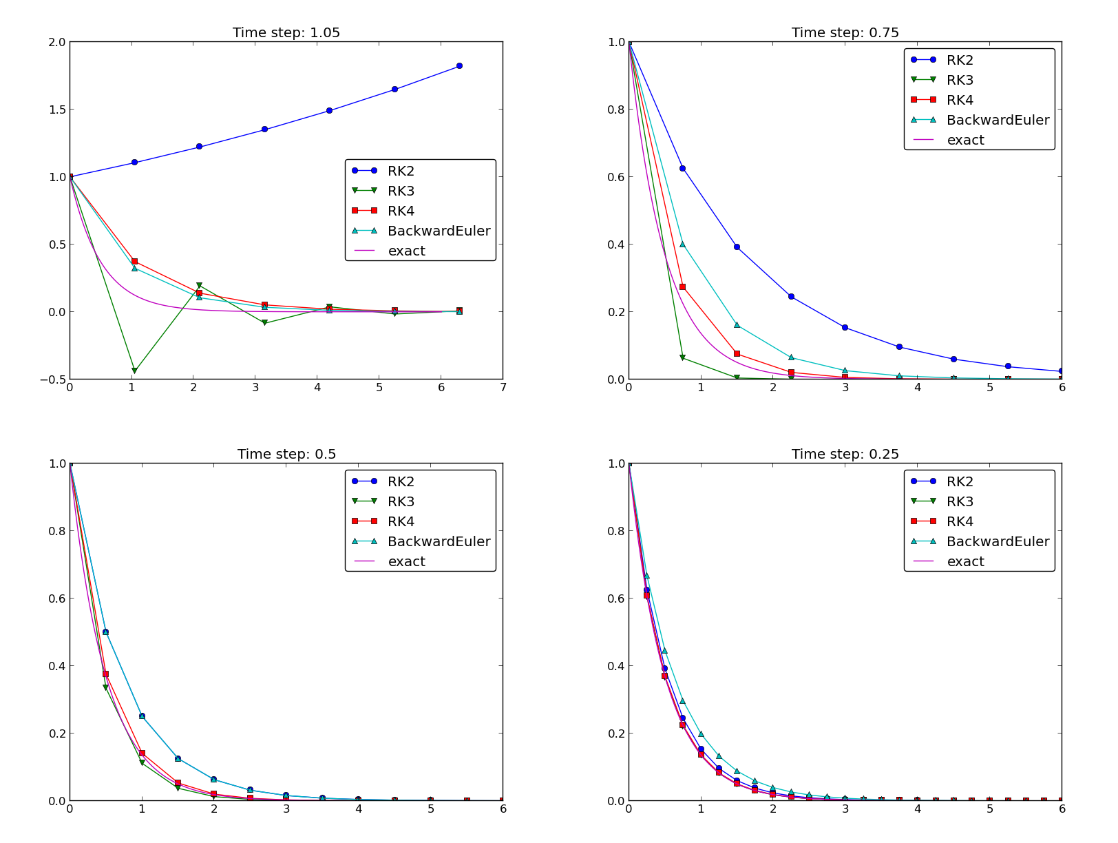
The 4-th order Runge-Kutta method (RK4) is the method of choice!
ode45).