$$
\newcommand{\uex}{{u_{\small\mbox{e}}}}
\newcommand{\Aex}{{A_{\small\mbox{e}}}}
\newcommand{\half}{\frac{1}{2}}
\newcommand{\Oof}[1]{\mathcal{O}(#1)}
$$
Example: Adaptive Runge-Kutta methods
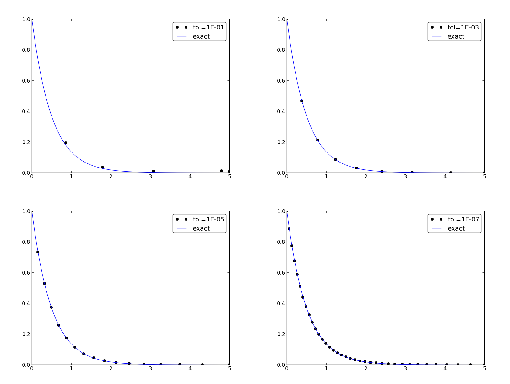
- Adaptive methods find "optimal" locations of the mesh points
to ensure that the error is less than a given tolerance.
- Downside: approximate error estimation, not always optimal
location of points.
- "Industry standard ODE solver": Dormand-Prince 4/5-th order
Runge-Kutta (MATLAB's famous
ode45).

