

(hpl 1: Need to cover functions, classes, modules, cml, GUI, hand calc, trivial problems, exact num sol, MMS, qualitative results, Git, bitbucket/github, scripting, report generation)
This problem is numerically solved by the so-called \( \theta \)-rule, which is a convenient way to merge different formulas for the well-known Forward Euler, Backward Euler, and Crank-Nicolson (midpoint/central) schemes. We introduce a uniform time mesh \( t_n=n\Delta t \), \( n=0,1,\ldots,N_t \), and seek \( u(t) \) at the mesh points. The numerical approximation to \( u(t_n) \) is denoted \( u^n \). Since we will use the symbol \( u \) both for the exact analytical solution of (1) and for the numerical approximation, we sometimes introduce \( \uex(t) \) to help distinguish the two types of solutions (i.e., subscript e for "exact") [1].
1: In the literature, it is more common to put a subscript
(like \( u_\Delta \) or \( u_h \))
on the numerical solution to distinguish it from the exact solution.
However, we will use the variable u in the code for the numerical
approximation to be computed, and therefore adjust the mathematical
notation to convenient conventions in the code such that we can have
as close correspondence as possible between the implementation and
the mathematics.
The \( \theta \)-rule leads to an explicit updating formula for \( u^{n+1} \), given \( u^n \):
(hpl 2: not ready. Need more here!!!!!!!)
from module import *
import module as m
Reading input data can be done in many ways. We have to decide on desired user interface, i.e., how we want to operate the program when providing input, and then use appropriate tools to implement the user interface. There are four basic types of user interface of relevance to our programs, listed here with increasing complexity of the implementation:
[[[
sys.argv, and there are, in principle, two ways of programming with
command-line arguments in Python:
sys.argv[1:] list (sys.argv[0] is
the just program name).--option value) on
the command line to override default values of input parameters,
and utilize the argparse.ArgumentParser tool to interact with
the command line.makeplot), and a list of \( \Delta t \) values.
The simplest way of reading this input from the command line is to say
that the first four command-line arguments correspond to the first
four points in the list above, in that order, and that the rest of the
command-line arguments are the \( \Delta t \) values. The input given for
makeplot can be a string among 'on', 'off', 'True', and
'False'. The code for reading this input is most conveniently put in
a function:
import sys

def read_command_line():
    if len(sys.argv) < 6:
        print 'Usage: %s I a T on/off dt1 dt2 dt3 ...' % \
              sys.argv[0]; sys.exit(1)  # abort

    I = float(sys.argv[1])
    a = float(sys.argv[2])
    T = float(sys.argv[3])
    makeplot = sys.argv[4] in ('on', 'True')
    dt_values = [float(arg) for arg in sys.argv[5:]]

    return I, a, T, makeplot, dt_values
One should note the following about the constructions in the program above:
sys.argv. Explicit conversion to, e.g., a float object is
required if the string as a number we want to compute with.makeplot is determined from a boolean expression,
which becomes True if the command-line argument is either 'on' or
'True', and False otherwise.sys.argv[5:], convert each command-line argument
to float, and collect these float objects in a list, using the
compact and convenient list comprehension syntax in Python.main function:
def main():
    I, a, T, makeplot, dt_values = read_command_line()
    for theta in 0, 0.5, 1:
        for dt in dt_values:
            E = explore(I, a, T, dt, theta, makeplot)
            print '%3.1f %6.2f: %12.3E' % (theta, dt, E)
The complete program can be found in decay_cml.py.
ArgumentParser tool in the argparse module makes it easy
to create a professional command-line interface to any program. The
documentation of ArgumentParser demonstrates its
versatile applications, so we shall here just list an example
containing basic features. On the command line we want to specify
option-value pairs for \( I \), \( a \), and \( T \), e.g., --a 3.5 --I 2 --T
2. Including --makeplot turns the plot on and excluding this option
turns the plot off. The \( \Delta t \) values can be given as --dt 1 0.5
0.25 0.1 0.01. Each parameter must have a sensible default value so
that we specify the option on the command line only when the default
value is not suitable.
We introduce a function for defining the mentioned command-line options:
def define_command_line_options():
    import argparse
    parser = argparse.ArgumentParser()
    parser.add_argument('--I', '--initial_condition', type=float,
                        default=1.0, help='initial condition, u(0)',
                        metavar='I')
    parser.add_argument('--a', type=float,
                        default=1.0, help='coefficient in ODE',
                        metavar='a')
    parser.add_argument('--T', '--stop_time', type=float,
                        default=1.0, help='end time of simulation',
                        metavar='T')
    parser.add_argument('--makeplot', action='store_true',
                        help='display plot or not')
    parser.add_argument('--dt', '--time_step_values', type=float,
                        default=[1.0], help='time step values',
                        metavar='dt', nargs='+', dest='dt_values')
    return parser
Each command-line option is defined through the parser.add_argument
method. Alternative options, like the short --I and the more
explaining version --initial_condition can be defined. Other arguments
are type for the Python object type, a default value, and a help
string, which gets printed if the command-line argument -h or --help is
included. The metavar argument specifies the value associated with
the option when the help string is printed. For example, the option for
\( I \) has this help output:
Terminal> python decay_argparse.py -h
  ...
  --I I, --initial_condition I
                        initial condition, u(0)
  ...
The structure of this output is
  --I metavar, --initial_condition metavar
                        help-string
The --makeplot option is a pure flag without any value, implying a
true value if the flag is present and otherwise a false value. The
action='store_true' makes an option for such a flag.
Finally, the --dt option demonstrates how to allow for more than one
value (separated by blanks) through the nargs='+' keyword argument.
After the command line is parsed, we get an object where the values of
the options are stored as attributes. The attribute name is specified
by the dist keyword argument, which for the --dt option is
dt_values. Without the dest argument, the value of an option --opt
is stored as the attribute opt.
The code below demonstrates how to read the command line and extract the values for each option:
def read_command_line():
    parser = define_command_line_options()
    args = parser.parse_args()
    print 'I={}, a={}, T={}, makeplot={}, dt_values={}'.format(
        args.I, args.a, args.T, args.makeplot, args.dt_values)
    return args.I, args.a, args.T, args.makeplot, args.dt_values
The main function remains the same as in the decay_cml.py code based
on reading from sys.argv directly. A complete program featuring the
demo above of ArgumentParser appears in the file decay_argparse.py.
decay_mod module with a GUI is quite technical
and of significantly less importance than knowing how to make
a command-line interface (the section Creating command-line interfaces).
There is no danger in jumping right to the section Computing convergence rates.
main function displayed in
the section ref{decay:plotting} for carrying out simulations and plotting
for a series of \( \Delta t \) values. Now we want to control and view the same
experiments from a web GUI.
To tell Parampool what type of input data we have,
we assign default values of the right type to all arguments in the
main function and call it main_GUI:
def main_GUI(I=1.0, a=.2, T=4.0,
         dt_values=[1.25, 0.75, 0.5, 0.1],
         theta_values=[0, 0.5, 1]):
The compute function must return the HTML code we want for displaying
the result in a web page. Here we want to show plots of the numerical
and exact solution for different methods and \( \Delta t \) values.
The plots can be organized in a table with \( \theta \) (methods) varying
through the columns and \( \Delta t \) varying through the rows.
Assume now that a new version of the explore function
not only returns the error E but also HTML code containing the
plot. Then we can write the main_GUI function as
def main_GUI(I=1.0, a=.2, T=4.0,
         dt_values=[1.25, 0.75, 0.5, 0.1],
         theta_values=[0, 0.5, 1]):
    # Build HTML code for web page. Arrange plots in columns
    # corresponding to the theta values, with dt down the rows
    theta2name = {0: 'FE', 1: 'BE', 0.5: 'CN'}
    html_text = '<table>\n'
    for dt in dt_values:
        html_text += '<tr>\n'
        for theta in theta_values:
            E, html = explore(I, a, T, dt, theta, makeplot=True)
            html_text += """
<td>
<center><b>%s, dt=%g, error: %s</b></center><br>
%s
</td>
""" % (theta2name[theta], dt, E, html)
        html_text += '</tr>\n'
    html_text += '</table>\n'
    return html_text
Rather than creating plot files and showing the plot on the screen,
the new version of the explore function makes a string with the PNG code of
the plot and embeds that string in HTML code. This action is
conveniently performed by Parampool's save_png_to_str function:
import matplotlib.pyplot as plt
...
# plot
plt.plot(t, u, r-')
plt.xlabel('t')
plt.ylabel('u')
...
from parampool.utils import save_png_to_str
html_text = save_png_to_str(plt, plotwidth=400)
Note that we now write plt.plot, plt.xlabel, etc.
The html_text string is long and contains all the characters that
build up the PNG file of the current plot. The new explore
function can make use of the above code snippet and return
html_text along with E.
from parampool.generator.flask import generate
from decay_GUI import main
generate(main,
         output_controller='decay_GUI_controller.py',
         output_template='decay_GUI_view.py',
         output_model='decay_GUI_model.py')
Running the decay_GUI_generate.py program results in three new
files whose names are specified in the call to generate:
decay_GUI_model.py defines HTML widgets to be used to set
input data in the web interface,templates/decay_GUI_views.py defines the layout of the web page,decay_GUI_controller.py runs the web application.
Terminal> python decay_GUI_controller.py
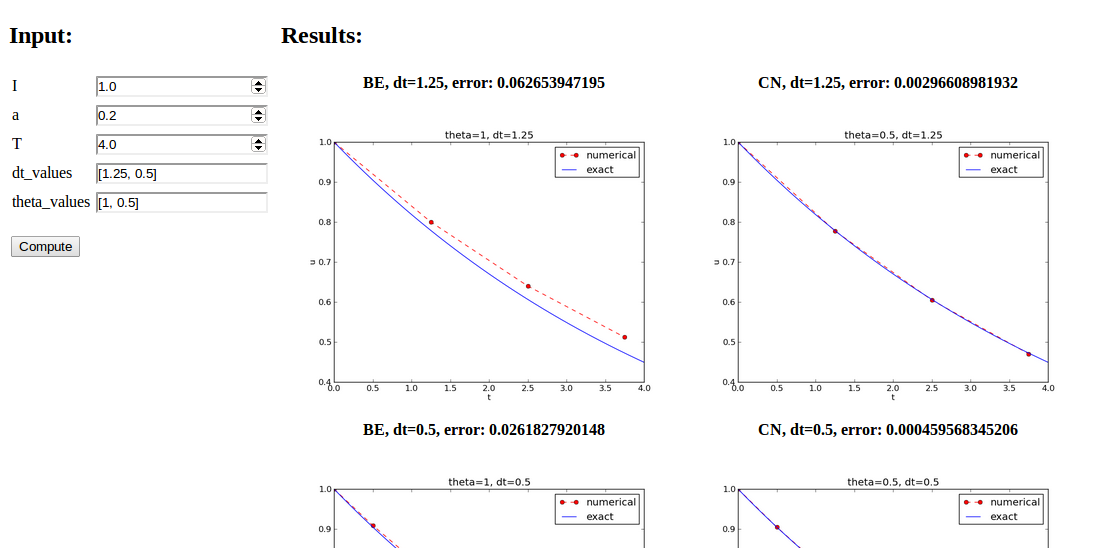
Open a web browser at the location 127.0.0.1:5000. Input fields for
I, a, T, dt_values, and theta_values are presented. Setting
the latter two to [1.25, 0.5] and [1, 0.5], respectively, and
pressing Compute results in four plots, see Figure
1. With the techniques demonstrated here, one can
easily create a tailored web GUI for a particular type of application
and use it to interactively explore physical and numerical effects.
Define $$ A = \frac{1 - (1-\theta) a\Delta t}{1 + \theta a \Delta t}\tp $$ Manual computations with the \( \theta \)-rule results in $$ \begin{align*} u^0 &= I,\\ u^1 &= Au^0 = AI,\\ u^2 &= Au^1 = A^2I,\\ &\vdots\\ u^n &= A^nu^{n-1} = A^nI \tp \end{align*} $$ We have then established the exact discrete solution as $$ \begin{equation} u^n = IA^n \tag{2} \tp \end{equation} $$
Comparison of the exact discrete solution and the computed solution is done in the following function:
def verify_exact_discrete_solution():

    def exact_discrete_solution(n, I, a, theta, dt):
        A = (1 - (1-theta)*a*dt)/(1 + theta*dt*a)
        return I*A**n

    theta = 0.8; a = 2; I = 0.1; dt = 0.8
    Nt = int(8/dt)  # no of steps
    u, t = solver(I=I, a=a, T=Nt*dt, dt=dt, theta=theta)
    u_de = array([exact_discrete_solution(n, I, a, theta, dt)
                  for n in range(Nt+1)])
    difference = abs(u_de - u).max()  # max deviation
    tol = 1E-15  # tolerance for comparing floats
    success = difference <= tol
    return success
The complete program is found in the file decay_verf2.py (verf2 is a short name for "verification,
version 2").
exact_discrete_solution does not need its five arguments as the
values can alternatively be accessed through the local variables defined
in the parent function verify_exact_discrete_solution. We can send
such an exact_discrete_solution without arguments to any other
function and exact_discrete_solution will still have access to
n, I, a, and so forth defined in its parent function.
The parameter \( r \) is known as the convergence rate. For example, if the convergence rate is 2, halving \( \Delta t \) reduces the error by a factor of 4. Diminishing \( \Delta t \) then has a greater impact on the error compared with methods that have \( r=1 \). For a given value of \( r \), we refer to the method as of \( r \)-th order. First- and second-order methods are most common in scientific computing.
The disadvantage of method 1 is that (3) might not be valid for the coarsest meshes (largest \( \Delta t \) values). Fitting a line to all the data points is then misleading. Method 2 computes convergence rates for pairs of experiments and allows us to see if the sequence \( r_i \) converges to some value as \( i\rightarrow m-2 \). The final \( r_{m-2} \) can then be taken as the convergence rate. If the coarsest meshes have a differing rate, the corresponding time steps are probably too large for (3) to be valid. That is, those time steps lie outside the asymptotic range of \( \Delta t \) values where the error behaves like (3).
main function in the program
decay_argparse.py with statements for computing \( r_0, r_1, \ldots, r_{m-2} \)
from (3):
from math import log

def main():
    I, a, T, makeplot, dt_values = read_command_line()
    r = {}  # estimated convergence rates
    for theta in 0, 0.5, 1:
        E_values = []
        for dt in dt_values:
            E = explore(I, a, T, dt, theta, makeplot=False)
            E_values.append(E)

        # Compute convergence rates
        m = len(dt_values)
        r[theta] = [log(E_values[i-1]/E_values[i])/
                    log(dt_values[i-1]/dt_values[i])
                    for i in range(1, m, 1)]

    for theta in r:
        print '\nPairwise convergence rates for theta=%g:' % theta
        print ' '.join(['%.2f' % r_ for r_ in r[theta]])
    return r
The program containing this main function is called decay_convrate.py.
The r object is a dictionary of lists. The keys in this
dictionary are the \( \theta \) values. For example,
r[1] holds the list of the \( r_i \) values corresponding to
\( \theta=1 \). In the loop for theta in r, the loop variable theta
takes on the values of the keys in the dictionary r (in an
undetermined ordering). We could simply do a print r[theta]
inside the loop, but this would typically yield output of
the convergence rates with 16 decimals:
[1.331919482274763, 1.1488178494691532, ...]
Instead, we format each number with 2 decimals, using a list
comprehension to turn the list of numbers, r[theta], into
a list of formatted strings. Then we join these strings
with a space in between to get a sequence of rates on one line
in the terminal window. More generally, d.join(list) joins the
strings in the list list to one string, with d
as delimiter between list[0], list[1], etc.
Here is an example on the outcome of the convergence rate computations:
Terminal> python decay_convrate.py --dt 0.5 0.25 0.1 0.05 0.025 0.01
...
Pairwise convergence rates for theta=0:
1.33 1.15 1.07 1.03 1.02

Pairwise convergence rates for theta=0.5:
2.14 2.07 2.03 2.01 2.01

Pairwise convergence rates for theta=1:
0.98 0.99 0.99 1.00 1.00
The Forward and Backward Euler methods seem to have an \( r \) value which stabilizes at 1, while the Crank-Nicolson seems to be a second-order method with \( r=2 \).
Very often, we have some theory that predicts what \( r \) is for a numerical method. Various theoretical error measures for the \( \theta \)-rule point to \( r=2 \) for \( \theta =0.5 \) and \( r=1 \) otherwise. The computed estimates of \( r \) are in very good agreement with these theoretical values.
a in the denominator
in the updating formula for u[n+1]:
u[n+1] = (1 - (1-theta)*a*dt)/(1 + theta*dt)*u[n]
Running the same decay_convrate.py command as above gives the expected
convergence rates (!). Why? The reason is that we just specified
the \( \Delta t \) values are relied on default values for other
parameters. The default value of \( a \) is 1. Forgetting the factor
a has then no effect. This example shows how important it is to
avoid parameters that are 1 or 0 when verifying implementations.
Running the code decay_v0.py with \( a=2.1 \) and \( I=0.1 \) yields
Terminal> python decay_convrate.py --a 2.1 --I 0.1  \
          --dt 0.5 0.25 0.1 0.05 0.025 0.01
...
Pairwise convergence rates for theta=0:
1.49 1.18 1.07 1.04 1.02

Pairwise convergence rates for theta=0.5:
-1.42 -0.22 -0.07 -0.03 -0.01

Pairwise convergence rates for theta=1:
0.21 0.12 0.06 0.03 0.01
This time we see that the expected convergence rates for the Crank-Nicolson and
Backward Euler methods are not obtained, while \( r=1 \) for the Forward Euler
method. The reason for correct rate in the latter case is that \( \theta=0 \)
and the wrong theta*dt term in the denominator vanishes anyway.
The error
u[n+1] = ((1-theta)*a*dt)/(1 + theta*dt*a)*u[n]
manifests itself through wrong rates \( r\approx 0 \) for all three methods.
About the same results arise from an erroneous initial condition, u[0] = 1,
or wrong loop limits, range(1,Nt). It seems that in this simple
problem, most bugs we can think of are detected by the convergence rate
test, provided the values of the input data do not hide the bug.
A verify_convergence_rate function could compute the dictionary of
list via main and check if the final rate estimates (\( r_{m-2} \))
are sufficiently close to the expected ones. A tolerance of 0.1
seems appropriate, given the uncertainty in estimating \( r \):
def verify_convergence_rate():
    r = main()
    tol = 0.1
    expected_rates = {0: 1, 1: 1, 0.5: 2}
    for theta in r:
        r_final = r[theta][-1]
        diff = abs(expected_rates[theta] - r_final)
        if diff > tol:
            return False
    return True  # all tests passed
We remark that r[theta] is a list and the last element in any list
can be extracted by the index -1.