Basic finite element methods
| Author: | Hans Petter Langtangen |
|---|---|
| Date: | Dec 12, 2012 |
Note: QUITE PRELIMINARY VERSION
The finite element method is a powerful tool for solving differential equations, especially in complicated domains and where higher-order approximations are desired. Figure Domain for flow around a dolphin shows a two-dimensional domain with a non-trivial geometry. The idea is to divide the domain into triangles (elements) and seek a polynomial approximations to the unknown functions on each triangle. The method glues these piecewise approximations together to find a global solution. Linear and quadratic polynomials over the triangles are particularly popular.
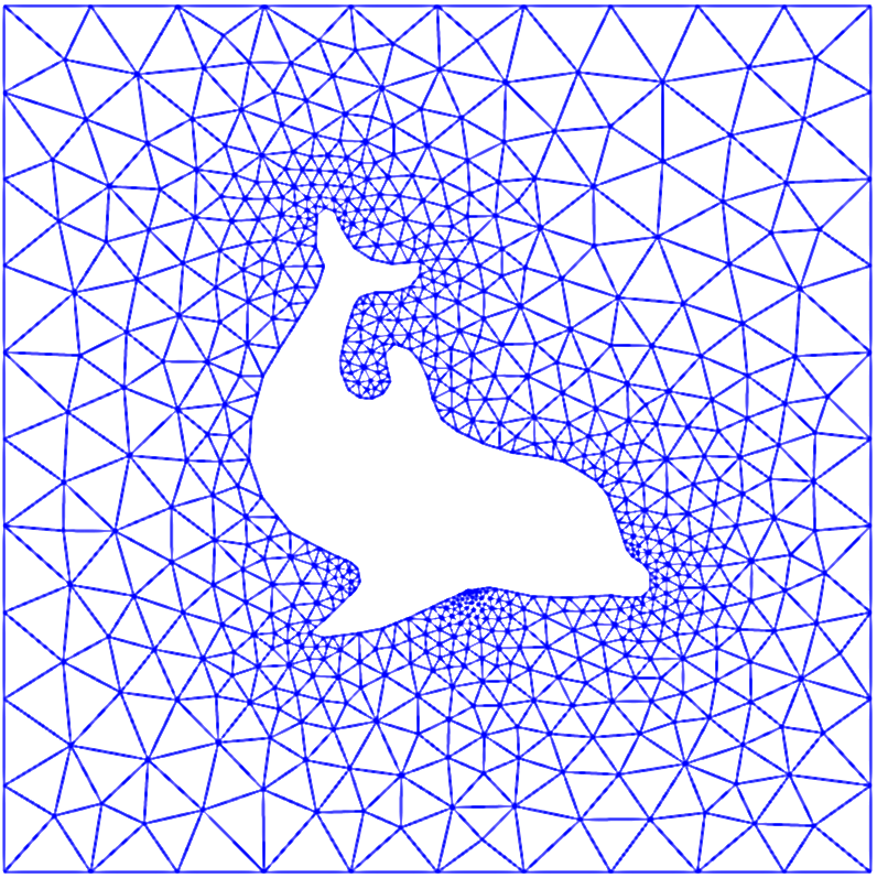
Domain for flow around a dolphin
Many successful numerical methods for differential equations, including the finite element method, aim at approximating the unknown function by a sum
where \({\varphi}_i(x)\) are prescribed functions and \(c_i\), \(i=0,\ldots,N\), are unknown coefficients to be determined. Solution methods for differential equations utilizing (1) must have a principle for constructing \(N+1\) equations to determine \(c_0,\ldots,c_N\). Then there is a machinery regarding the actual constructions of the equations for \(c_0,\ldots,c_N\) in a particular problem. Finally, there is a solve phase for computing the solution \(c_0,\ldots,c_N\) of the \(N+1\) equations.
Especially in the finite element method, the machinery for constructing the discrete equations to be implemented on a computer is quite comprehensive, with many mathematical and implementational details entering the scene at the same time. From an ease-of-learning perspective it can therefore be wise to introduce the computational machinery for a trivial equation: \(u=f\). Solving this equation with \(f\) given and \(u\) on the form (1) means that we seek an approximation \(u\) to \(f\). This approximation problem has the advantage of introducing most of the finite element toolbox, but with postponing demanding topics related to differential equations (e.g., integration by parts, boundary conditions, and coordinate mappings). This is the reason why we shall first become familiar with finite element approximation before addressing finite element methods for differential equations.
First, we refresh some linear algebra concepts about approximating vectors in vector spaces. Second, we extend these concepts to approximating functions in function spaces, using the same principles and the same notation. We present examples on approximating functions by global basis functions with support throughout the entire domain. Third, we introduce the finite element type of local basis functions and explain the computational algorithms for working with such functions. Three types of approximation principles are covered: 1) the least squares method, 2) the Galerkin or \(L_2\) projection method, and 3) interpolation or collocation.
Approximation of vectors
We shall start with introducing two fundamental methods for determining the coefficients \(c_i\) in (1) and illustrate the methods on approximation of vectors, because vectors in vector spaces is more intuitive than working with functions in function spaces. The extension from vectors to functions will be trivial as soon as the fundamental ideas are understood.
The first method of approximation is called the least squares method and consists in finding \(c_i\) such that the difference \(u-f\), measured in some norm, is minimized. That is, we aim at finding the best approximation \(u\) to \(f\) (in some norm). The second method is not as intuitive: we find \(u\) such that the error \(u-f\) is orthogonal to the space where we seek \(u\). This is known as projection, or we may also call it a Galerkin method. When approximating vectors and functions, the two methods are equivalent, but this is no longer the case when working with differential equations.
Approximation of planar vectors
Suppose we have given a vector \(\pmb{f} = (3,5)\) in the \(xy\) plane and that we want to approximate this vector by a vector aligned in the direction of the vector \((a,b)\). Figure Approximation of a two-dimensional vector by a one-dimensional vector depicts the situation.
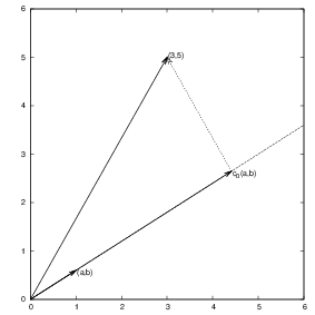
Approximation of a two-dimensional vector by a one-dimensional vector
We introduce the vector space \(V\) spanned by the vector \(\pmb{\varphi}_0=(a,b)\):
We say that \(\pmb{\varphi}_0\) is a basis vector in the space \(V\). Our aim is to find the vector \(\pmb{u} = c_0\pmb{\varphi}_0\in V\) which best approximates the given vector \(\pmb{f} = (3,5)\). A reasonable criterion for a best approximation could be to minimize the length of the difference between the approximate \(\pmb{u}\) and the given \(\pmb{f}\). The difference, or error, \(\pmb{e} = \pmb{f} -\pmb{u}\) has its length given by the norm
where \((\pmb{e},\pmb{e})\) is the inner product of \(\pmb{e}\) and itself. The inner product, also called scalar product or dot product, of two vectors \(\pmb{u}=(u_0,u_1)\) and \(\pmb{v} =(v_0,v_1)\) is defined as
Remark 1. We should point out that we use the notation \((\cdot,\cdot)\) for two different things: \((a,b)\) for scalar quantities \(a\) and \(b\) means the vector starting in the origin and ending in the point \((a,b)\), while \((\pmb{u},\pmb{v})\) with vectors \(\pmb{u}\) and \(\pmb{v}\) means the inner product of these vectors. Since vectors are here written in boldface font there should be no confusion. Note that the norm associated with this inner product is the usual Eucledian length of a vector.
Remark 2. It might be wise to refresh some basic linear algebra by consulting a textbook. Exercise 1: Linear algebra refresher I and Exercise 2: Linear algebra refresher II suggest specific tasks to regain familiarity with fundamental operations on inner product vector spaces.
The least squares method (1)
We now want to find \(c_0\) such that it minimizes \(||\pmb{e}||\). The algebra is simplified if we minimize the square of the norm, \(||\pmb{e}||^2 = (\pmb{e}, \pmb{e})\). Define
We can rewrite the expressions of the right-hand side to a more convenient form for further work:
The rewrite results from using the following fundamental rules for inner product spaces:
Minimizing \(E(c_0)\) implies finding \(c_0\) such that
Differentiating (2) with respect to \(c_0\) gives
Setting the above expression equal to zero and solving for \(c_0\) gives
which in the present case with \(\pmb{\varphi}_0=(a,b)\) results in
For later, it is worth mentioning that setting the key equation (3) to zero can be rewritten as
or
The Galerkin or projection method (1)
Minimizing \(||\pmb{e}||^2\) implies that \(\pmb{e}\) is orthogonal to any vector \(\pmb{v}\) in the space \(V\). This result is visually quite clear from Figure Approximation of a two-dimensional vector by a one-dimensional vector (think of other vectors along the line \((a,b)\): all of them will lead to a larger distance between the approximation and \(\pmb{f}\)). To see this result mathematically, we express any \(\pmb{v}\in V\) as \(\pmb{v}=s\pmb{\varphi}_0\) for any scalar parameter \(s\), recall that two vectors are orthogonal when their inner product vanishes, and calculate the inner product
Therefore, instead of minimizing the square of the norm, we could demand that \(\pmb{e}\) is orthogonal to any vector in \(V\). This approach is known as projection, because we it is the same as projecting the vector onto the subspace. We may also use the term Galerkin’s method. Mathematically the approach is stated by the equation
Since an arbitrary \(\pmb{v}\in V\) can be expressed as \(s\pmb{\varphi}_0\), \(s\in\mathbb{R}\), (6) implies
which means that the error must be orthogonal to the basis vector in the space \(V\):
The latter equation gives (4) for \(c_0\). Furthermore, the latter equation also arose from least squares computations in (5).
Approximation of general vectors
Let us generalize the vector approximation from the previous section to vectors in spaces with arbitrary dimension. Given some vector \(\pmb{f}\), we want to find the best approximation to this vector in the space
We assume that the basis vectors \(\pmb{\varphi}_0,\ldots,\pmb{\varphi}_N\) are linearly independent so that none of them are redundant and the space has dimension \(N+1\). Any vector \(\pmb{u}\in V\) can be written as a linear combination of the basis vectors,
where \(c_j\in\mathbb{R}\) are scalar coefficients to be determined.
The least squares method (2)
Now we want to find \(c_0,\ldots,c_N\) such that \(\pmb{u}\) is the best approximation to \(\pmb{f}\) in the sense that the distance, or error, \(\pmb{e} = \pmb{f} - \pmb{u}\) is minimized. Again, we define the squared distance as a function of the free parameters \(c_0,\ldots,c_N\),
Minimizing this \(E\) with respect to the independent variables \(c_0,\ldots,c_N\) is obtained by setting
The second term in (7) is differentiated as follows:
since the expression to be differentiated is a sum and only one term, \(c_i(\pmb{f},\pmb{\varphi}_i)\), contains \(c_i\) and this term is linear in \(c_i\). To understand this differentiation in detail, write out the sum specifically for, e.g, \(N=3\) and \(i=1\).
The last term in (7) is more tedious to differentiate. We start with
Then
The last term can be included in the other two sums, resulting in
It then follows that setting
leads to a linear system for \(c_0,\ldots,c_N\):
where
(Note that we can change the order of the two vectors in the inner product as desired.)
The Galerkin or projection method (2)
In analogy with the “one-dimensional” example in the section Approximation of planar vectors, it holds also here in the general case that minimizing the distance (error) \(\pmb{e}\) is equivalent to demanding that \(\pmb{e}\) is orthogonal to all \(\pmb{v}\in V\):
Since any \(\pmb{v}\in V\) can be written as \(\pmb{v} =\sum_{i=0}^N c_i\pmb{\varphi}_i\), the statement (9) is equivalent to saying that
for any choice of coefficients \(c_0,\ldots,c_N\in\mathbb{R}\). The latter equation can be rewritten as
If this is to hold for arbitrary values of \(c_0,\ldots,c_N\), we must require that each term in the sum vanishes,
These \(N+1\) equations result in the same linear system as (8):
and hence
So, instead of differentiating the \(E(c_0,\ldots,c_N)\) function, we could simply use (9) as the principle for determining \(c_0,\ldots,c_N\), resulting in the \(N+1\) equations (10).
The names least squares method or least squares approximation are natural since the calculations consists of minimizing \(||\pmb{e}||^2\), and \(||\pmb{e}||^2\) is a sum of squares of differences between the components in \(\pmb{f}\) and \(\pmb{u}\). We find \(\pmb{u}\) such that this sum of squares is minimized.
The principle (9), or the equivalent form (10), is known as projection. Almost the same mathematical idea was used by the Russian mathematician Boris Galerkin to solve differential equations, resulting in what is widely known as Galerkin’s method.
Approximation of functions
Let \(V\) be a function space spanned by a set of basis functions \({\varphi}_0,\ldots,{\varphi}_N\),
such that any function \(u\in V\) can be written as a linear combination of the basis functions:
For now, in this introduction, we shall look at functions of a single variable \(x\): \(u=u(x)\), \({\varphi}_i={\varphi}_i(x)\), \(i=0,\ldots,N\). Later, we will extend the scope to functions of two- or three-dimensional physical spaces. The approximation (11) is typically used to discretize a problem in space. Other methods, most notably finite differences, are common for time discretization (although the form (11) can be used in time too).
The least squares method (3)
Given a function \(f(x)\), how can we determine its best approximation \(u(x)\in V\)? A natural starting point is to apply the same reasoning as we did for vectors in the section Approximation of general vectors. That is, we minimize the distance between \(u\) and \(f\). However, this requires a norm for measuring distances, and a norm is most conveniently defined through an inner product. Viewing a function as a vector of infinitely many point values, one for each value of \(x\), the inner product could intuitively be defined as the usual summation of pairwise components, with summation replaced by integration:
To fix the integration domain, we let \(f(x)\) and \({\varphi}_i(x)\) be defined for a domain \(\Omega\subset\mathbb{R}\). The inner product of two functions \(f(x)\) and \(g(x)\) is then
The distance between \(f\) and any function \(u\in V\) is simply \(f-u\), and the squared norm of this distance is
Note the analogy with (7): the given function \(f\) plays the role of the given vector \(\pmb{f}\), and the basis function \({\varphi}_i\) plays the role of the basis vector \(\pmb{\varphi}_i\). We get can rewrite (13), through similar steps as used for the result (7), leading to
Minimizing this function of \(N+1\) scalar variables \(c_0,\ldots,c_N\) requires differentiation with respect to \(c_i\), for \(i=0,\ldots,N\). The resulting equations are very similar to those we had in the vector case, and we hence end up with a linear system of the form (8), with
The Galerkin or projection method (3)
As in the section Approximation of general vectors, the minimization of \((e,e)\) is equivalent to
This is known as a projection of a function \(f\) onto the subspace \(V\). We may also call it a Galerkin method for approximating functions. Using the same reasoning as in (9)-(10), it follows that (14) is equivalent to
Inserting \(e=f-u\) in this equation and ordering terms, as in the multi-dimensional vector case, we end up with a linear system with a coefficient matrix (?) and right-hand side vector (?).
Whether we work with vectors in the plane, general vectors, or functions in function spaces, the least squares principle and the Galerkin or projection method are equivalent.
Example: linear approximation
Let us apply the theory in the previous section to a simple problem: given a parabola \(f(x)=10(x-1)^2-1\) for \(x\in\Omega=[1,2]\), find the best approximation \(u(x)\) in the space of all linear functions:
That is, \({\varphi}_0(x)=1\), \({\varphi}_1(x)=x\), and \(N=1\). We seek
where \(c_0\) and \(c_1\) are found by solving a \(2\times 2\) the linear system. The coefficient matrix has elements
The corresponding right-hand side is
Solving the linear system results in
and consequently
Figure Best approximation of a parabola by a straight line displays the parabola and its best approximation in the space of all linear functions.
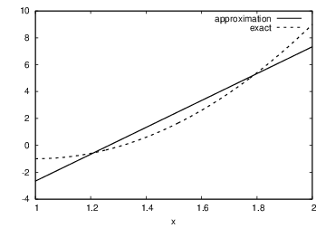
Best approximation of a parabola by a straight line
Implementation of the least squares method
The linear system can be computed either symbolically or numerically (a numerical integration rule is needed in the latter case). Here is a function for symbolic computation of the linear system, where \(f(x)\) is given as a sympy expression f (involving the symbol x), phi is a list of \({\varphi}_0,\ldots,{\varphi}_N\), and Omega is a 2-tuple/list holding the domain \(\Omega\):
import sympy as sm

def least_squares(f, phi, Omega):
    N = len(phi) - 1
    A = sm.zeros((N+1, N+1))
    b = sm.zeros((N+1, 1))
    x = sm.Symbol('x')
    for i in range(N+1):
        for j in range(i, N+1):
            A[i,j] = sm.integrate(phi[i]*phi[j],
                                  (x, Omega[0], Omega[1]))
            A[j,i] = A[i,j]
        b[i,0] = sm.integrate(phi[i]*f, (x, Omega[0], Omega[1]))
    c = A.LUsolve(b)
    u = 0
    for i in range(len(phi)):
        u += c[i,0]*phi[i]
    return u
Observe that we exploit the symmetry of the coefficient matrix: only the upper triangular part is computed. Symbolic integration in sympy is often time consuming, and (roughly) halving the work has noticeable effect on the waiting time for the function to finish execution.
Comparing the given \(f(x)\) and the approximate \(u(x)\) visually is done by the following function, which with the aid of sympy‘s lambdify tool converts a sympy functional expression to a Python function for numerical computations:
def comparison_plot(f, u, Omega, filename='tmp.pdf'):
    x = sm.Symbol('x')
    f = sm.lambdify([x], f, modules="numpy")
    u = sm.lambdify([x], u, modules="numpy")
    resolution = 401  # no of points in plot
    xcoor  = linspace(Omega[0], Omega[1], resolution)
    exact  = f(xcoor)
    approx = u(xcoor)
    plot(xcoor, approx)
    hold('on')
    plot(xcoor, exact)
    legend(['approximation', 'exact'])
    savefig(filename)
The modules='numpy' argument to lambdify is important if there are mathematical functions, such as sin or exp in the symbolic expressions in f or u, and these mathematical functions are to be used with vector arguments, like xcoor above.
Both the least_squares and comparison_plot are found and coded in the file approx1D.py. The forthcoming examples on their use appear in ex_approx1D.py.
Perfect approximation
Let us use the code above to recompute the problem from the section Example: linear approximation where we want to approximate a parabola. What happens if we add an element \(x^2\) to the basis and test what the best approximation is if \(V\) is the space of all parabolic functions? The answer is quickly found by running
>>> from approx1D import *
>>> x = sm.Symbol('x')
>>> f = 10*(x-1)**2-1
>>> u = least_squares(f=f, phi=[1, x, x**2], Omega=[1, 2])
>>> print u
10*x**2 - 20*x + 9
>>> print sm.expand(f)
10*x**2 - 20*x + 9
Now, what if we use \(\phi_i(x)=x^i\) for \(i=0,\ldots,N=40\)? The output from least_squares gives \(c_i=0\) for \(i>2\). In fact, we have a general result that if \(f\in V\), the least squares and Galerkin/projection methods compute the exact solution \(u=f\).
The proof is straightforward: if \(f\in V\), \(f\) can be expanded in terms of the basis functions, \(f=\sum_{j=0}^Nd_j{\varphi}_j\), for some coefficients \(d_0,\ldots,d_N\), and the right-hand side then has entries
The linear system \(\sum_jA_{i,j}c_j = b_i\), \(i=0,\ldots,N\), is then
which implies that \(c_i=d_i\) for \(i=0,\ldots,N\).
Ill-conditioning
The computational example in the section Perfect approximation applies the least_squares function which invokes symbolic methods to calculate and solve the linear system. The correct solution \(c_0=9, c_1=-20, c_2=10, c_i=0\) for \(i\geq 3\) is perfectly recovered.
Suppose we convert the matrix and right-hand side to floating-point arrays and then solve the system using finite-precision arithmetics, which is what one will (almost) always do in real life. This time we get astonishing results! Up to about \(N=7\) we get a solution that is reasonably close to the exact one. Increasing \(N\) shows that seriously wrong coefficients are computed. Below is a table showing the solution of the linear system arising from approximating a parabola by functions on the form \(u(x)=\sum_{j=0}^Nc_jx^j\), \(N=10\). Analytically, we know that \(c_j=0\) for \(j>2\), but ill-conditioning may produce \(c_j\neq 0\) for \(j>2\).
| exact | sympy | numpy32 | numpy64 |
|---|---|---|---|
| 9 | 9.62 | 5.57 | 8.98 |
| -20 | -23.39 | -7.65 | -19.93 |
| 10 | 17.74 | -4.50 | 9.96 |
| 0 | -9.19 | 4.13 | -0.26 |
| 0 | 5.25 | 2.99 | 0.72 |
| 0 | 0.18 | -1.21 | -0.93 |
| 0 | -2.48 | -0.41 | 0.73 |
| 0 | 1.81 | -0.013 | -0.36 |
| 0 | -0.66 | 0.08 | 0.11 |
| 0 | 0.12 | 0.04 | -0.02 |
| 0 | -0.001 | -0.02 | 0.002 |
The exact value of \(c_j\), \(j=0,\ldots,10\), appears in the first column while the other columns correspond to results obtained by three different methods:
- Column 2: The matrix and vector are converted to the data structure sympy.mpmath.fp.matrix and the sympy.mpmath.fp.lu_solve function is used to solve the system.
- Column 3: The matrix and vector are converted to numpy arrays with data type numpy.float32 (single precision floating-point number) and solved by the numpy.linalg.solve function.
- Column 4: As column 3, but the data type is numpy.float64 (double precision floating-point number).
We see from the numbers in the table that double precision performs much better than single precision. Nevertheless, when plotting all these solutions the curves cannot be visually distinguished (!). This means that the approximations look perfect, despite the partially wrong values of the coefficients.
Increasing \(N\) to 12 makes the numerical solver in sympy report abort with the message: “matrix is numerically singular”. A matrix has to be non-singular to be invertible, which is a requirement when solving a linear system. Already when the matrix is close to singular, it is ill-conditioned, which here implies that the numerical solution algorithms are sensitive to round-off errors and may produce (very) inaccurate results.
The reason why the coefficient matrix is nearly singular and ill-conditioned is that our basis functions \({\varphi}_i(x)=x^i\) are nearly linearly dependent for large \(i\). That is, \(x^i\) and \(x^{i+1}\) are very close for \(i\) not very small. This phenomenon is illustrated in Figure The 15 first basis functions , . There are 15 lines in this figure, but only half of them are visually distinguishable. Almost linearly dependent basis functions give rise to an ill-conditioned and almost singular matrix. This fact can be illustrated by computing the determinant, which is indeed very close to zero (recall that a zero determinant implies a singular and non-invertible matrix): \(10^{-65}\) for \(N=10\) and \(10^{-92}\) for \(N=12\). Already for \(N=28\) the numerical determinant computation returns a plain zero.
The 15 first basis functions \(x^i\), \(i=0,\ldots,14\)
On the other hand, the double precision numpy solver do run for \(N=100\), resulting in answers that are not significantly worse than those in the table above, and large powers are associated with small coefficients (e.g., \(c_j<10^{-2}\) for \(10\leq j\leq 20\) and \(c<10^{-5}\) for \(j>20\)). Even for \(N=100\) the approximation lies on top of the exact curve in a plot (!).
The conclusion is that visual inspection of the quality of the approximation may not uncover fundamental numerical problems with the computations. However, numerical analysts have studied approximations and ill-conditioning for decades, and it is well known that the basis \(\{1,x,x^2,x^3,\ldots,\}\) is a bad basis. The best basis from a matrix conditioning point of view is to have orthogonal functions such that \((\phi_i,\phi_j)=0\) for \(i\neq j\). There are many known sets of orthogonal polynomials. The functions used in the finite element methods are almost orthogonal, and this property helps to avoid problems with solving matrix systems. Almost orthogonal is helpful, but not enough when it comes to partial differential equations, and ill-conditioning of the coefficient matrix is a theme when solving large-scale finite element systems.
Fourier series
A set of sine functions is widely used for approximating functions. Let us take
That is,
An approximation to the \(f(x)\) function from the section Example: linear approximation can then be computed by the least_squares function from the section Implementation of the least squares method:
N = 3
from sympy import sin, pi
x = sm.Symbol('x')
phi = [sin(pi*(i+1)*x) for i in range(N+1)]
f = 10*(x-1)**2 - 1
Omega = [0, 1]
u = least_squares(f, phi, Omega)
comparison_plot(f, u, Omega)
Figure Best approximation of a parabola by a sum of 3 (left) and 11 (right) sine functions (left) shows the oscillatory approximation of \(\sum_{j=0}^{N}c_j\sin ((j+1)\pi x)\) when \(N=3\). Changing \(N\) to 11 improves the approximation considerably, see Figure Best approximation of a parabola by a sum of 3 (left) and 11 (right) sine functions (right).
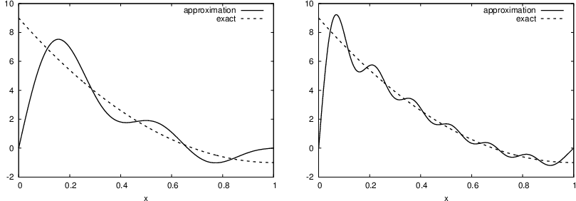
Best approximation of a parabola by a sum of 3 (left) and 11 (right) sine functions
There is an error \(f(0)-u(0)=9\) at \(x=0\) in Figure Best approximation of a parabola by a sum of 3 (left) and 11 (right) sine functions regardless of how large \(N\) is, because all \({\varphi}_i(0)=0\) and hence \(u(0)=0\). We may help the approximation to be correct at \(x=0\) by seeking
However, this adjustments introduces a new problem at \(x=1\) since we now get an error \(f(1)-u(1)=f(1)-0=-1\) at this point. A more clever adjustment is to replace the \(f(0)\) term by a term that is \(f(0)\) at \(x=0\) and \(f(1)\) at \(x=1\). A simple linear combination \(f(0)(1-x) + xf(1)\) does the job:
This adjustment of \(u\) alters the linear system slightly as we get an extra term \(-(f(0)(1-x) + xf(1),{\varphi}_i)\) on the right-hand side. Figure Best approximation of a parabola by a sum of 3 (left) and 11 (right) sine functions with a boundary term shows the result of ensuring right boundary values: even 3 sines can now adjust the \(f(0)(1-x) + xf(1)\) term such that \(u\) approximates the parabola really well, at least visually.
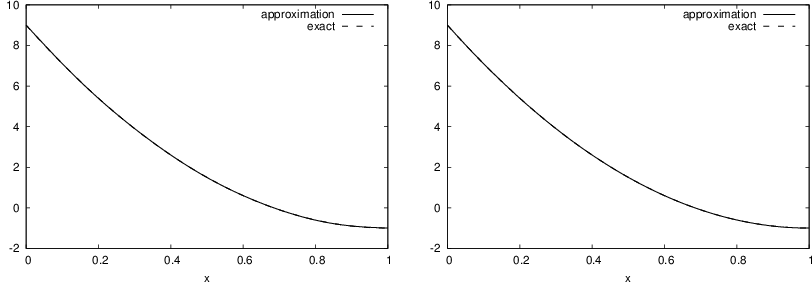
Best approximation of a parabola by a sum of 3 (left) and 11 (right) sine functions with a boundary term
Orthogonal basis functions
The choice of sine functions \({\varphi}_i(x)=\sin ((i+1)\pi x)\) has a great computational advantage: on \(\Omega=[0,1]\) these basis functions are orthogonal, implying that \(A_{i,j}=0\) if \(i\neq j\). This result is realized by trying
integrate(sin(j*pi*x)*sin(k*pi*x), x, 0, 1)
in WolframAlpha (avoid i in the integrand as this symbol means the imaginary unit \(\sqrt{-1}\)). Also by asking WolframAlpha about \(\int_0^1\sin^2 (j\pi x) dx\), we find it to equal 1/2. With a diagonal matrix we can easily solve for the coefficients by hand:
which is nothing but the classical formula for the coefficients of the Fourier sine series of \(f(x)\) on \([0,1]\). In fact, when \(V\) contains the basic functions used in a Fourier series expansion, the approximation method derived in the section Approximation of functions results in the classical Fourier series for \(f(x)\) (see Exercise 6: Fourier series as a least squares approximation for details).
For orthogonal basis functions we can make the least_squares function (much) more efficient since we know that the matrix is diagonal and only the diagonal elements need to be computed:
def least_squares_orth(f, phi, Omega):
    N = len(phi) - 1
    A = [0]*(N+1)
    b = [0]*(N+1)
    x = sm.Symbol('x')
    for i in range(N+1):
        A[i] = sm.integrate(phi[i]**2, (x, Omega[0], Omega[1]))
        b[i] = sm.integrate(phi[i]*f,  (x, Omega[0], Omega[1]))
    c = [b[i]/A[i] for i in range(len(b))]
    u = 0
    for i in range(len(phi)):
        u += c[i]*phi[i]
    return u
This function is found in the file approx1D.py.
The collocation (interpolation) method
The principle of minimizing the distance between \(u\) and \(f\) is an intuitive way of computing a best approximation \(u\in V\) to \(f\). However, there are other attractive approaches as well. One is to demand that \(u(x_{i}) = f(x_{i})\) at some selected points \(x_{i}\), \(i=0,\ldots,N\):
This criterion also gives a linear system with \(N+1\) unknown coefficients \(c_0,\ldots,c_N\):
with
This time the coefficient matrix is not symmetric because \({\varphi}_j(x_{i})\neq {\varphi}_i(x_{j})\) in general. The method is often referred to as a collocation method and the \(x_{i}\) points are known as collocation points. Others view the approach as an interpolation method since some point values of \(f\) are given (\(f(x_{i})\)) and we fit a continuous function \(u\) that goes through the \(f(x_{i})\) points. In that case the \(x_{i}\) points are called interpolation points.
Given \(f\) as a sympy symbolic expression f, \({\varphi}_0,\ldots,{\varphi}_N\) as a list phi, and a set of points \(x_0,\ldots,x_N\) as a list or array points, the following Python function sets up and solves the matrix system for the coefficients \(c_0,\ldots,c_N\):
def interpolation(f, phi, points):
    N = len(phi) - 1
    A = sm.zeros((N+1, N+1))
    b = sm.zeros((N+1, 1))
    x = sm.Symbol('x')
    # Turn phi and f into Python functions
    phi = [sm.lambdify([x], phi[i]) for i in range(N+1)]
    f = sm.lambdify([x], f)
    for i in range(N+1):
        for j in range(N+1):
            A[i,j] = phi[j](points[i])
        b[i,0] = f(points[i])
    c = A.LUsolve(b)
    u = 0
    for i in range(len(phi)):
        u += c[i,0]*phi[i](x)
    return u
Note that it is convenient to turn the expressions f and phi into Python functions which can be called with elements of points as arguments when building the matrix and the right-hand side. The interpolation function is a part of the approx1D module.
A nice feature of the interpolation or collocation method is that it avoids computing integrals. However, one has to decide on the location of the \(x_{i}\) points. A simple, yet common choice, is to distribute them uniformly throughout \(\Omega\).
Example (1)
Let us illustrate the interpolation or collocation method by approximating our parabola \(f(x)=10(x-1)^2-1\) by a linear function on \(\Omega=[1,2]\), using two collocation points \(x_0=1+1/3\) and \(x_1=1+2/3\):
f = 10*(x-1)**2 - 1
phi = [1, x]
Omega = [1, 2]
points = [1 + sm.Rational(1,3), 1 + sm.Rational(2,3)]
u = interpolation(f, phi, points)
comparison_plot(f, u, Omega)
The resulting linear system becomes
with solution \(c_0=-119/9\) and \(c_1=10\). Figure Approximation of a parabola by linear functions computed by two interpolation points: 4/3 and 5/3 (left) versus 1 and 2 (right) (left) shows the resulting approximation \(u=-119/9 + 10x\). We can easily test other interpolation points, say \(x_0=1\) and \(x_1=2\). This changes the line quite significantly, see Figure Approximation of a parabola by linear functions computed by two interpolation points: 4/3 and 5/3 (left) versus 1 and 2 (right) (right).
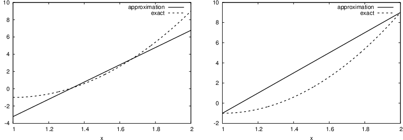
Approximation of a parabola by linear functions computed by two interpolation points: 4/3 and 5/3 (left) versus 1 and 2 (right)
Lagrange polynomials
In the section Fourier series we explain the advantage with having a diagonal matrix: formulas for the coefficients \(c_0,\ldots,c_N\) can then be derived by hand. For an interpolation/collocation method a diagonal matrix implies that \({\varphi}_j(x_{i}) = 0\) if \(i\neq j\). One set of basis functions \({\varphi}_i(x)\) with this property is the Lagrange interpolating polynomials, or just Lagrange polynomials. (Although the functions are named after Lagrange, they were first discovered by Waring in 1779, rediscovered by Euler in 1783, and published by Lagrange in 1795.) The Lagrange polynomials have the form
for \(i=0,\ldots,N\). We see from (16) that all the \({\varphi}_i\) functions are polynomials of degree \(N\) which have the property
when \(x_s\) is an interpolation/collocation point. This property implies that \(A_{i,j}=0\) for \(i\neq j\) and \(A_{i,j}=1\) when \(i=j\). The solution of the linear system is them simply
and
The following function computes the Lagrange interpolating polynomial \({\varphi}_i(x)\), given the interpolation points \(x_{0},\ldots,x_{N}\) in the list or array points:
def Lagrange_polynomial(x, i, points):
    p = 1
    for k in range(len(points)):
        if k != i:
            p *= (x - points[k])/(points[i] - points[k])
    return p
The next function computes a complete basis using equidistant points throughout \(\Omega\):
def Lagrange_polynomials_01(x, N):
    if isinstance(x, sm.Symbol):
        h = sm.Rational(1, N-1)
    else:
        h = 1.0/(N-1)
    points = [i*h for i in range(N)]
    phi = [Lagrange_polynomial(x, i, points) for i in range(N)]
    return phi, points
When x is an sm.Symbol object, we let the spacing between the interpolation points, h, be a sympy rational number for nice end results in the formulas for \({\varphi}_i\). The other case, when x is a plain Python float, signifies numerical computing, and then we let h be a floating-point number. Observe that the Lagrange_polynomial function works equally well in the symbolic and numerical case (think of x being an sm.Symbol object or a Python float). A little interactive session illustrates the difference between symbolic and numerical computing of the basis functions and points:
>>> import sympy as sm
>>> x = sm.Symbol('x')
>>> phi, points = Lagrange_polynomials_01(x, N=3)
>>> points
[0, 1/2, 1]
>>> phi
[(1 - x)*(1 - 2*x), 2*x*(2 - 2*x), -x*(1 - 2*x)]

>>> x = 0.5  # numerical computing
>>> phi, points = Lagrange_polynomials_01(x, N=3, symbolic=True)
>>> points
[0.0, 0.5, 1.0]
>>> phi
[-0.0, 1.0, 0.0]
The Lagrange polynomials are very much used in finite element methods because of their property (17).
Successful example
Trying out the Lagrange polynomial basis for approximating \(f(x)=\sin 2\pi x\) on \(\Omega =[0,1]\) with the least squares and the interpolation techniques can be done by
x = sm.Symbol('x')
f = sm.sin(2*sm.pi*x)
phi, points = Lagrange_polynomials_01(x, N)
Omega=[0, 1]
u = least_squares(f, phi, Omega)
comparison_plot(f, u, Omega)
u = interpolation(f, phi, points)
comparison_plot(f, u, Omega)
Figure Approximation via least squares (left) and interpolation (right) of a sine function by Lagrange interpolating polynomials of degree 4 shows the results. There is little difference between the least squares and the interpolation technique. Increasing \(N\) gives visually better approximations.
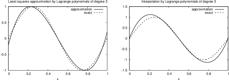
Approximation via least squares (left) and interpolation (right) of a sine function by Lagrange interpolating polynomials of degree 4
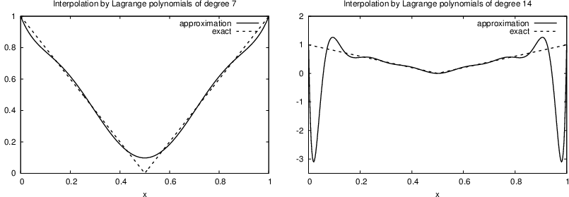
Less successful example
The next example concerns interpolating \(f(x)=|1-2x|\) on \(\Omega =[0,1]\) using Lagrange polynomials. Figure Interpolation of an absolute value function by Lagrange polynomials and uniformly distributed interpolation points: degree 7 (left) and 14 (right) shows a peculiar effect: the approximation starts to oscillate more and more as \(N\) grows. This numerical artifact is not surprising when looking at the individual Lagrange polynomials: Figure Illustration of the oscillatory behavior of two Lagrange polynomials for 12 uniformly spaced points (marked by circles) shows two such polynomials of degree 11, and it is clear that the basis functions oscillate significantly. The reason is simple, since we force the functions to be 1 at one point and 0 at many other points. A polynomial of high degree is then forced to oscillate between these points. The oscillations are particularly severe at the boundary. The phenomenon is named Runge’s phenomenon and you can read
a more detailed explanation on Wikipedia.
Remedy for strong oscillations
The oscillations can be reduced by a more clever choice of interpolation points, called the Chebyshev nodes:
on the interval \(\Omega = [a,b]\). Here is a flexible version of the Lagrange_polynomials_01 function above, valid for any interval \(\Omega =[a,b]\) and with the possibility to generate both uniformly distributed points and Chebyshev nodes:
def Lagrange_polynomials(x, N, Omega, point_distribution='uniform'):
    if point_distribution == 'uniform':
        if isinstance(x, sm.Symbol):
            h = sm.Rational(Omega[1] - Omega[0], N)
        else:
            h = (Omega[1] - Omega[0])/float(N)
        points = [Omega[0] + i*h for i in range(N+1)]
    elif point_distribution == 'Chebyshev':
        points = Chebyshev_nodes(Omega[0], Omega[1], N)
    phi = [Lagrange_polynomial(x, i, points) for i in range(N+1)]
    return phi, points

def Chebyshev_nodes(a, b, N):
    from math import cos, pi
    return [0.5*(a+b) + 0.5*(b-a)*cos(float(2*i+1)/(2*(N+1))*pi) \
            for i in range(N+1)]
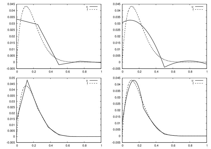
All the functions computing Lagrange polynomials listed above are found in the module file Lagrange.py. Figure Interpolation of an absolute value function by Lagrange polynomials and Chebyshev nodes as interpolation points: degree 7 (left) and 14 (right) shows the improvement of using Chebyshev nodes (compared with Figure Interpolation of an absolute value function by Lagrange polynomials and uniformly distributed interpolation points: degree 7 (left) and 14 (right)).
Another cure for undesired oscillation of higher-degree interpolating polynomials is to use lower-degree Lagrange polynomials on many small patches of the domain, which is the idea pursued in the finite element method. For instance, linear Lagrange polynomials on \([0,1/2]\) and \([1/2,1]\) would yield a perfect approximation to \(f(x)=|1-2x|\) on \(\Omega = [0,1]\) since \(f\) is piecewise linear.
Interpolation of an absolute value function by Lagrange polynomials and uniformly distributed interpolation points: degree 7 (left) and 14 (right)
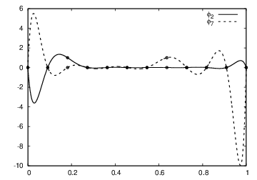
Illustration of the oscillatory behavior of two Lagrange polynomials for 12 uniformly spaced points (marked by circles)
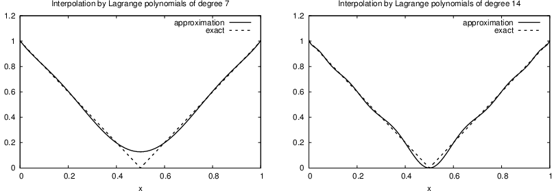
Interpolation of an absolute value function by Lagrange polynomials and Chebyshev nodes as interpolation points: degree 7 (left) and 14 (right)
Unfortunately, sympy has problems integrating the \(f(x)=|1-2x|\) function times a polynomial. Other choices of \(f(x)\) can also make the symbolic integration fail. Therefore, we should extend the least_squares function such that it falls back on numerical integration if the symbolic integration is unsuccessful. In the latter case, the returned value from sympy‘s integrate function is an object of type Integral. We can test on this type and utilize the mpmath module in sympy to perform numerical integration of high precision. Here is the code:
def least_squares(f, phi, Omega):
    N = len(phi) - 1
    A = sm.zeros((N+1, N+1))
    b = sm.zeros((N+1, 1))
    x = sm.Symbol('x')
    for i in range(N+1):
        for j in range(i, N+1):
            integrand = phi[i]*phi[j]
            I = sm.integrate(integrand, (x, Omega[0], Omega[1]))
            if isinstance(I, sm.Integral):
                # Could not integrate symbolically, fallback
                # on numerical integration with mpmath.quad
                integrand = sm.lambdify([x], integrand)
                I = sm.mpmath.quad(integrand, [Omega[0], Omega[1]])
            A[i,j] = A[j,i] = I
        integrand = phi[i]*f
        I = sm.integrate(integrand, (x, Omega[0], Omega[1]))
        if isinstance(I, sm.Integral):
            integrand = sm.lambdify([x], integrand)
            I = sm.mpmath.quad(integrand, [Omega[0], Omega[1]])
        b[i,0] = I
    c = A.LUsolve(b)
    u = 0
    for i in range(len(phi)):
        u += c[i,0]*phi[i]
    return u
Finite element basis functions
The specific basis functions exemplified in the section Approximation of functions are in general nonzero on the entire domain \(\Omega\), see Figure Approximation based on sine basis functions for an example. We shall now turn the attention to basis functions that have compact support, meaning that they are nonzero on only a small portion of \(\Omega\). Moreover, we shall restrict the functions to be piecewise polynomials. This means that the domain is split into subdomains and the function is a polynomial on one or more subdomains, see Figure Approximation based on local piecewise linear (hat) functions for a sketch involving locally defined hat functions that make \(u=\sum_jc_j{\varphi}_j\) piecewise linear. At the boundaries between subdomains one normally forces continuity of the function only so that when connecting two polynomials from two subdomains, the derivative usually becomes discontinuous. These type of basis functions are fundamental in the finite element method.
Approximation based on sine basis functions
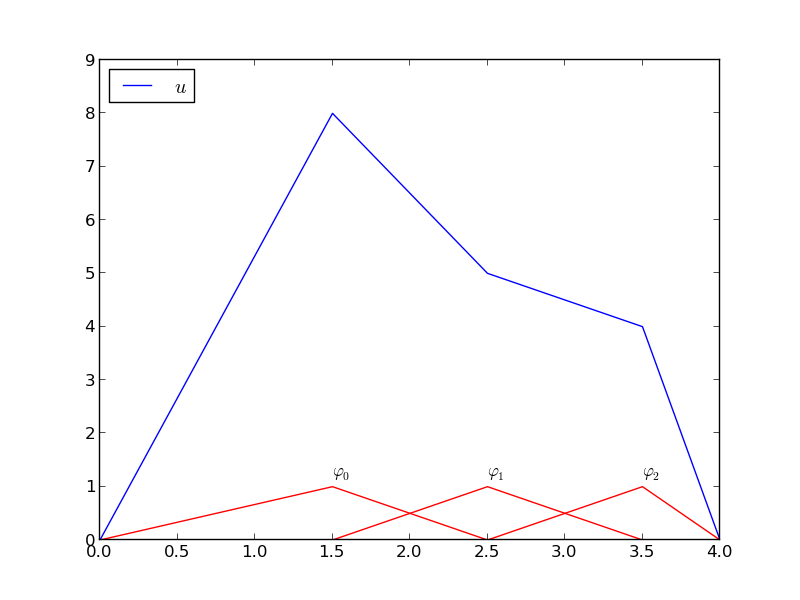
Approximation based on local piecewise linear (hat) functions
We first introduce the concepts of elements and nodes in a simplistic fashion as often met in the literature. Later, we shall generalize the concept of an element, which is a necessary step to treat a wider class of approximations within the family of finite element methods. The generalization is also compatible with the concepts used in the FEniCS finite element software.
Elements and nodes
Let us divide the interval \(\Omega\) on which \(f\) and \(u\) are defined into non-overlapping subintervals \(\Omega^{(e)}\), \(e=0,\ldots,n_e\):
We shall for now refer to \(\Omega^{(e)}\) as an element, having number \(e\). On each element we introduce a set of points called nodes. For now we assume that the nodes are uniformly spaced throughout the element and that the boundary points of the elements are also nodes. The nodes are given numbers both within an element and in the global domain. These are referred to as local and global node numbers, respectively.
Nodes and elements uniquely define a finite element mesh, which is our discrete representation of the domain in the computations. .. index:: finite element mesh
A common special case is that of a uniformly partitioned mesh where each element has the same length and the distance between nodes is constant.
Example (2)
On \(\Omega =[0,1]\) we may introduce two elements, \(\Omega^{(0)}=[0,0.4]\) and \(\Omega^{(1)}=[0.4,1]\). Furthermore, let us introduce three nodes per element, equally spaced within each element. The three nodes in element number 0 are \(x_0=0\), \(x_1=0.2\), and \(x_2=0.4\). The local and global node numbers are here equal. In element number 1, we have the local nodes \(x_0=0.4\), \(x_1=0.7\), and \(x_2=1\) and the corresponding global nodes \(x_2=0.4\), \(x_3=0.7\), and \(x_4=1\). Note that the global node \(x_2=0.4\) is shared by the two elements.
For the purpose of implementation, we introduce two lists or arrays: nodes for storing the coordinates of the nodes, with the global node numbers as indices, and elements for holding the global node numbers in each element, with the local node numbers as indices. The nodes and elements lists for the sample mesh above take the form
nodes = [0, 0.2, 0.4, 0.7, 1]
elements = [[0, 1, 2], [2, 3, 4]]
Looking up the coordinate of local node number 2 in element 1 is here done by nodes[elements[1][2]] (recall that nodes and elements start their numbering at 0).
The basis functions
Construction principles
Standard finite element basis functions are now defined as follows. Let \(i\) be the global node number corresponding to local node \(r\) in element number \(e\).
- If local node number \(r\) is not on the boundary of the element, take \({\varphi}_i(x)\) to be the Lagrange polynomial that is 1 at the local node number \(r\) and zero at all other nodes in the element. On all other elements, \({\varphi}_i=0\).
- If local node number \(r\) is on the boundary of the element, let \({\varphi}_i\) be made up of the Lagrange polynomial that is 1 at this node in element number \(e\) and its neighboring element. On all other elements, \({\varphi}_i=0\).
A visual impression of three such basis functions are given in Figure fem:approx:fe:fig:P2. Sometimes we refer to a Lagrange polynomial on an element \(e\), which means the basis function \({\varphi}_i(x)\) when \(x\in\Omega^{(e)}\), and \({\varphi}_i(x)=0\) when \(x\notin\Omega^{(e)}\).
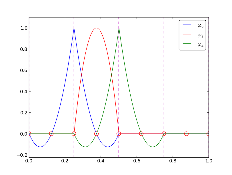
Illustration of the piecewise quadratic basis functions associated with nodes in element 1
Properties of \({\varphi}_i\)
The construction of basis functions according to the principles above lead to two important properties of \({\varphi}_i(x)\). First,
when \(x_{j}\) is a node in the mesh with global node number \(j\), because the Lagrange polynomials are constructed to have this property. The property also implies a convenient interpretation of \(c_i\) as the value of \(u\) at node \(i\):
Because of this interpretation, the coefficient \(c_i\) is by many named \(u_i\) or \(U_i\).
Second, \({\varphi}_i(x)\) is mostly zero throughout the domain:
- \({\varphi}_i(x) \neq 0\) only on those elements that contain global node \(i\),
- \({\varphi}_i(x){\varphi}_j(x) \neq 0\) if and only if \(i\) and \(j\) are global node numbers in the same element.
Since \(A_{i,j}\) is the integral of \({\varphi}_i{\varphi}_j\) it means that most of the elements in the coefficient matrix will be zero. We will come back to these properties and use them actively in computations to save memory and CPU time.
We let each element have \(d+1\) nodes, resulting in local Lagrange polynomials of degree \(d\). It is not a requirement to have the same \(d\) value in each element, but for now we will assume so.
Example on quadratic \({\varphi}_i\)
Figure fem:approx:fe:fig:P2 illustrates how piecewise quadratic basis functions can look like (\(d=2\)). We work with the domain \(\Omega = [0,1]\) divided into four equal-sized elements, each having three nodes. The nodes and elements lists in this particular example become
nodes = [0, 0.125, 0.25, 0.375, 0.5, 0.625, 0.75, 0.875, 1.0]
elements = [[0, 1, 2], [2, 3, 4], [4, 5, 6], [6, 7, 8]]
Nodes are marked with circles on the \(x\) axis in the figure, and element boundaries are marked with vertical dashed lines.
Illustration of the piecewise quadratic basis functions associated with nodes in element 1
Let us explain in detail how the basis functions are constructed according to the principles. Consider element number 1 in Figure fem:approx:fe:fig:P2, \(\Omega^{(1)}=[0.25, 0.5]\), with local nodes 0, 1, and 2 corresponding to global nodes 2, 3, and 4. The coordinates of these nodes are \(0.25\), \(0.375\), and \(0.5\), respectively. We define three Lagrange polynomials on this element:
- The polynomial that is 1 at local node 1 (\(x=0.375\), global node 3) makes up the basis function \({\varphi}_3(x)\) over this element, with \({\varphi}_3(x)=0\) outside the element.
- The Lagrange polynomial that is 1 at local node 0 is the “right part” of the global basis function \({\varphi}_2(x)\). The “left part” of \({\varphi}_2(x)\) consists of a Lagrange polynomial associated with local node 2 in the neighboring element \(\Omega^{(0)}=[0, 0.25]\).
- Finally, the polynomial that is 1 at local node 2 (global node 4) is the “left part” of the global basis function \({\varphi}_4(x)\). The “right part” comes from the Lagrange polynomial that is 1 at local node 0 in the neighboring element \(\Omega^{(2)}=[0.5, 0.75]\).
As mentioned earlier, any global basis function \({\varphi}_i(x)\) is zero on elements that do not share the node with global node number \(i\).
The other global functions associated with internal nodes, \({\varphi}_1\), \({\varphi}_5\), and \({\varphi}_7\), are all of the same shape as the drawn \({\varphi}_3\), while the global basis functions associated with shared nodes also have the same shape, provided the elements are of the same length.
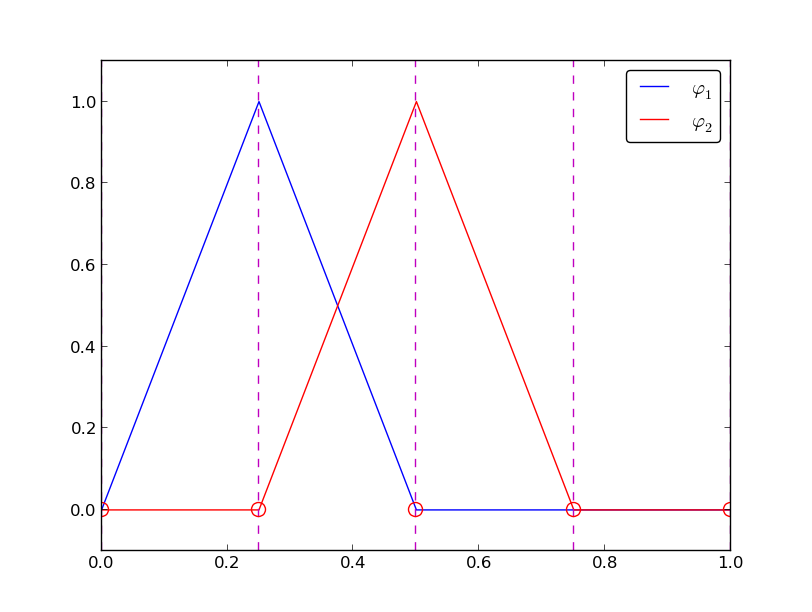
Illustration of the piecewise linear basis functions associated with nodes in element 1
Example on linear \({\varphi}_i\)
Figure Illustration of the piecewise linear basis functions associated with nodes in element 1 shows piecewise linear basis functions (\(d=1\)). Also here we have four elements on \(\Omega = [0,1]\). Consider the element \(\Omega^{(1)}=[0.25,0.5]\). Now there are no internal nodes in the elements so that all basis functions are associated with nodes at the element boundaries and hence made up of two Lagrange polynomials from neighboring elements. For example, \({\varphi}_1(x)\) results from the Lagrange polynomial in element 0 that is 1 at local node 1 and 0 at local node 0, combined with the Lagrange polynomial in element 1 that is 1 at local node 0 and 0 at local node 1. The other basis functions are constructed similarly.
Explicit mathematical formulas are needed for \({\varphi}_i(x)\) in computations. In the piecewise linear case, one can show that
Here, \(x_{j}\), \(j=i-1,i,i+1\), denotes the coordinate of node \(j\). For elements of equal length \(h\) the formulas can be simplified to
Example on cubic \({\varphi}_i\)
Piecewise cubic basis functions can be defined by introducing four nodes per element. Figure Illustration of the piecewise cubic basis functions associated with nodes in element 1 shows examples on \({\varphi}_i(x)\), \(i=3,4,5,6\), associated with element number 1. Note that \({\varphi}_4\) and \({\varphi}_5\) are nonzero on element number 1, while \({\varphi}_3\) and \({\varphi}_6\) are made up of Lagrange polynomials on two neighboring elements.
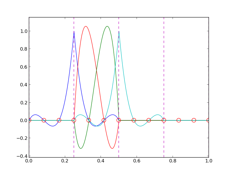
Illustration of the piecewise cubic basis functions associated with nodes in element 1
We see that all the piecewise linear basis functions have the same “hat” shape. They are naturally referred to as hat functions, also called chapeau functions. The piecewise quadratic functions in Figure fem:approx:fe:fig:P2 are seen to be of two types. “Rounded hats” associated with internal nodes in the elements and some more “sombrero” shaped hats associated with element boundary nodes. Higher-order basis functions also have hat-like shapes, but the functions have pronounced oscillations in addition, as illustrated in Figure Illustration of the piecewise cubic basis functions associated with nodes in element 1.
A common terminology is to speak about linear elements as elements with two local nodes and where the basis functions are piecewise linear. Similarly, quadratic elements and cubic elements refer to piecewise quadratic or cubic functions over elements with three or four local nodes, respectively. Alternative names, frequently used later, are P1 elements for linear elements, P2 for quadratic elements, and so forth (P$d$ signifies degree \(d\) of the polynomial basis functions).
Calculating the linear system
The elements in the coefficient matrix and right-hand side, given by the formulas (?) and (?), will now be calculated for piecewise polynomial basis functions. Consider P1 (piecewise linear) elements. Nodes and elements numbered consecutively from left to right imply the nodes \(x_i=i h\) and the elements
We have in this case \(N\) elements and \(N+1\) nodes, and \(\Omega=[x_{0},x_{N}]\). The formula for \({\varphi}_i(x)\) is given by (20) and a graphical illustration is provided in Figure Illustration of the piecewise linear basis functions associated with nodes in element 1. First we clearly see from Figure Illustration of the piecewise linear basis functions associated with nodes in element 1 that the important property \({\varphi}_i(x){\varphi}_j(x)\neq 0\) if and only if \(j=i-1\), \(j=i\), or \(j=i+1\), or alternatively expressed, if and only if \(i\) and \(j\) are nodes in the same element. Otherwise, \({\varphi}_i\) and \({\varphi}_j\) are too distant to have an overlap and consequently a nonzero product.
The element \(A_{i,i-1}\) in the coefficient matrix can be calculated as
It turns out that \(A_{i,i+1} =h/6\) as well and that \(A_{i,i}=2h/3\). The numbers are modified for \(i=0\) and \(i=N\): \(A_{0,0}=h/3\) and \(A_{N,N}=h/3\). The general formula for the right-hand side becomes
With two equal-sized elements in \(\Omega=[0,1]\) and \(f(x)=x(1-x)\), one gets
The solution becomes
The resulting function
is displayed in Figure Least squares approximation using 2 (left) and 4 (right) P1 elements (left). Doubling the number of elements to four leads to the improved approximation in the right part of Figure Least squares approximation using 2 (left) and 4 (right) P1 elements.
Least squares approximation using 2 (left) and 4 (right) P1 elements
Assembly of elementwise computations
The integrals are naturally split into integrals over individual elements since the formulas change with the elements. This idea of splitting the integral is fundamental in all practical implementations of the finite element method.
Let us split the integral over \(\Omega\) into a sum of contributions from each element:
Now, \(A^{(e)}_{i,j}\neq 0\) if and only if \(i\) and \(j\) are nodes in element \(e\). Introduce \(i=q(e,r)\) as the mapping of local node number \(r\) in element \(e\) to the global node number \(i\). This is just a short mathematical notation for the expression i=elements[e][r] in a program. Let \(r\) and \(s\) be the local node numbers corresponding to the global node numbers \(i=q(e,r)\) and \(j=q(e,s)\). With \(d\) nodes per element, all the nonzero elements in \(A^{(e)}_{i,j}\) arise from the integrals involving basis functions with indices corresponding to the global node numbers in element number \(e\):
These contributions can be collected in a \((d+1)\times (d+1)\) matrix known as the element matrix. We introduce the notation
for the element matrix. For the case \(d=2\) we have
Given the numbers \(\tilde A^{(e)}_{r,s}\), we should according to (22) add the contributions to the global coefficient matrix by
This process of adding in elementwise contributions to the global matrix is called finite element assembly or simply assembly. .. index:: assembly
Figure Illustration of matrix assembly illustrates how element matrices for elements with two nodes are added into the global matrix. More specifically, the figure shows how the element matrix associated with elements 2 and 3 assembled, assuming that global nodes are numbered from left to right in the domain.
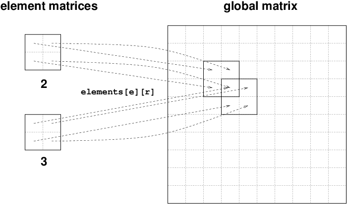
Illustration of matrix assembly
The right-hand side of the linear system is also computed elementwise:
We observe that \(b_i^{(e)}\neq 0\) if and only if global node \(i\) is a node in element \(e\). With \(d\) nodes per element we can collect the \(d+1\) nonzero contributions \(b_i^{(e)}\), for \(i=q(e,r)\), \(r=0,\ldots,d\), in an element vector
These contributions are added to the global right-hand side by an assembly process similar to that for the element matrices:
Mapping to a reference element
Instead of computing the integrals
over some element \(\Omega^{(e)} = [x_L, x_R]\), it is convenient to map the element domain \([x_L, x_R]\) to a standardized reference element domain \([-1,1]\). (We have now introduced \(x_L\) and \(x_R\) as the left and right boundary points of an arbitrary element. With a natural numbering of nodes and elements from left to right through the domain, \(x_L=x_{e}\) and \(x_R=x_{e+1}\).) Let \(X\) be the coordinate in the reference element. A linear or affine mapping from \(X\) to \(x\) reads
This relation can alternatively be expressed by
where we have introduced the element midpoint \(x_m=(x_L+x_R)/2\) and the element length \(h=x_R-x_L\).
Integrating on the reference element is a matter of just changing the integration variable from \(x\) to \(X\). Let
be the basis function associated with local node number \(r\) in the reference element. The integral transformation reads
The stretch factor \(dx/dX\) between the \(x\) and \(X\) coordinates becomes the determinant of the Jacobian matrix of the mapping between the coordinate systems in 2D and 3D. To obtain a uniform notation for 1D, 2D, and 3D problems we therefore replace \(dx/dX\) by \(\det J\) already now. In 1D, \(\det J = dx/dX = h/2\). The integration over the reference element is then written as
The corresponding formula for the element vector entries becomes
Since we from now on will work in the reference element, we need explicit mathematical formulas for the basis functions \({\varphi}_i(x)\) in the reference element only, i.e., we only need to specify formulas for \({\tilde{\varphi}}_r(X)\). This is a very convenient simplification compared to specifying piecewise polynomials in the physical domain.
The \({\tilde{\varphi}}_r(x)\) functions are simply the Lagrange polynomials defined through the local nodes in the reference element. For \(d=1\) and two nodes per element, we have the linear Lagrange polynomials
Quadratic polynomials, \(d=2\), have the formulas
In general,
where \(X_{(0)},\ldots,X_{(d)}\) are the coordinates of the local nodes in the reference element. These are normally uniformly spaced: \(X_{(r)} = -1 + 2r/d\), \(r=0,\ldots,d\).
Integration over a reference element
To illustrate the concepts from the previous section in a specific example, we now consider calculation of the element matrix and vector for a specific choice of \(d\) and \(f(x)\). A simple choice is \(d=1\) and \(f(x)=x(1-x)\) on \(\Omega =[0,1]\). We have the general expressions (25) and (26) for \(\tilde A^{(e)}_{r,s}\) and \(\tilde b^{(e)}_{r}\). Writing these out for the choices (?) and (?), and using that \(\det J = h/2\), we get
In the last two expressions we have used the element midpoint \(x_m\).
Integration of lower-degree polynomials above is tedious, and higher-degree polynomials that very much more algebra, but sympy may help. For example,
>>> import sympy as sm
>>> x, x_m, h, X = sm.symbols('x x_m h X')
>>> sm.integrate(h/8*(1-X)**2, (X, -1, 1))
h/3
>>> sm.integrate(h/8*(1+X)*(1-X), (X, -1, 1))
h/6
>>> x = x_m + h/2*X
>>> b_0 = sm.integrate(h/4*x*(1-x)*(1-X), (X, -1, 1))
>>> print b_0
-h**3/24 + h**2*x_m/6 - h**2/12 - h*x_m**2/2 + h*x_m/2
For inclusion of formulas in documents (like the present one), sympy can print expressions in LaTeX format:
>>> print sm.latex(b_0, mode='plain')
- \frac{1}{24} h^{3} + \frac{1}{6} h^{2} x_{m}
- \frac{1}{12} h^{2} - \frac{1}{2} h x_{m}^{2}
+ \frac{1}{2} h x_{m}
Implementation (1)
Based on the experience from the previous example, it makes sense to write some code to automate the integration process for any choice of finite element basis functions. In addition, we can automate the assembly process and linear system solution. Appropriate functions for this purpose document all details of all steps in the finite element computations and can found in the module file fe_approx1D.py. Some of the functions are explained below.
Integration
First we need a Python function for defining \({\tilde{\varphi}}_r(X)\) in terms of a Lagrange polynomial of degree d:
import sympy as sm
import numpy as np

def phi_r(r, X, d):
    if isinstance(X, sm.Symbol):
        h = sm.Rational(1, d)  # node spacing
        nodes = [2*i*h - 1 for i in range(d+1)]
    else:
        # assume X is numeric: use floats for nodes
        nodes = np.linspace(-1, 1, d+1)
    return Lagrange_polynomial(X, r, nodes)

def Lagrange_polynomial(x, i, points):
    p = 1
    for k in range(len(points)):
        if k != i:
            p *= (x - points[k])/(points[i] - points[k])
    return p
Observe how we construct the phi_r function to be a symbolic expression for \({\tilde{\varphi}}_r(X)\) if X is a Symbol object from sympy. Otherwise, we assume that X is a float object and compute the corresponding floating-point value of \({\tilde{\varphi}}_r(X)\). The Lagrange_polynomial function, copied here from the section Fourier series, works with both symbolic and numeric x and points variables.
The complete basis \({\tilde{\varphi}}_0(X),\ldots,{\tilde{\varphi}}_d(X)\) on the reference element is constructed by
def basis(d=1):
    X = sm.Symbol('X')
    phi = [phi_r(r, X, d) for r in range(d+1)]
    return phi
Now we are in a position to write the function for computing the element matrix:
def element_matrix(phi, Omega_e, symbolic=True):
    n = len(phi)
    A_e = sm.zeros((n, n))
    X = sm.Symbol('X')
    if symbolic:
        h = sm.Symbol('h')
    else:
        h = Omega_e[1] - Omega_e[0]
    detJ = h/2  # dx/dX
    for r in range(n):
        for s in range(r, n):
            A_e[r,s] = sm.integrate(phi[r]*phi[s]*detJ, (X, -1, 1))
            A_e[s,r] = A_e[r,s]
    return A_e
In the symbolic case (symbolic is True), we introduce the element length as a symbol h in the computations. Otherwise, the real numerical value of the element interval Omega_e is used and the final matrix elements are numbers, not symbols. This functionality can be demonstrated:
>>> from fe_approx1D import *
>>> phi = basis(d=1)
>>> phi
[1/2 - X/2, 1/2 + X/2]
>>> element_matrix(phi, Omega_e=[0.1, 0.2], symbolic=True)
[h/3, h/6]
[h/6, h/3]
>>> element_matrix(phi, Omega_e=[0.1, 0.2], symbolic=False)
[0.0333333333333333, 0.0166666666666667]
[0.0166666666666667, 0.0333333333333333]
The computation of the element vector is done by a similar procedure:
def element_vector(f, phi, Omega_e, symbolic=True):
    n = len(phi)
    b_e = sm.zeros((n, 1))
    # Make f a function of X
    X = sm.Symbol('X')
    if symbolic:
        h = sm.Symbol('h')
    else:
        h = Omega_e[1] - Omega_e[0]
    x = (Omega_e[0] + Omega_e[1])/2 + h/2*X  # mapping
    f = f.subs('x', x)  # substitute mapping formula for x
    detJ = h/2  # dx/dX
    for r in range(n):
        b_e[r] = sm.integrate(f*phi[r]*detJ, (X, -1, 1))
    return b_e
Here we need to replace the symbol x in the expression for f by the mapping formula such that f contains the variable X.
The integration in the element matrix function involves only products of polynomials, which sympy can easily deal with, but for the right-hand side sympy may face difficulties with certain types of expressions f. The result of the integral is then an Integral object and not a number as when symbolic integration is successful. It may therefore be wise to introduce a fallback on numerical integration. The symbolic integration can also take much time before an unsuccessful conclusion so we may introduce a parameter symbolic and set it to False to avoid symbolic integration:
def element_vector(f, phi, Omega_e, symbolic=True):
        ...
        if symbolic:
            I = sm.integrate(f*phi[r]*detJ, (X, -1, 1))
        if not symbolic or isinstance(I, sm.Integral):
            h = Omega_e[1] - Omega_e[0]  # Ensure h is numerical
            detJ = h/2
            integrand = sm.lambdify([X], f*phi[r]*detJ)
            I = sm.mpmath.quad(integrand, [-1, 1])
        b_e[r] = I
        ...
Successful numerical integration requires that the symbolic integrand is converted to a plain Python function (integrand) and that the element length h is a real number.
Linear system assembly and solution
The complete algorithm for computing and assembling the elementwise contributions takes the following form
def assemble(nodes, elements, phi, f, symbolic=True):
    n_n, n_e = len(nodes), len(elements)
    if symbolic:
        A = sm.zeros((n_n, n_n))
        b = sm.zeros((n_n, 1))    # note: (n_n, 1) matrix
    else:
        A = np.zeros((n_n, n_n))
        b = np.zeros(n_n)
    for e in range(n_e):
        Omega_e = [nodes[elements[e][0]], nodes[elements[e][-1]]]

        A_e = element_matrix(phi, Omega_e, symbolic)
        b_e = element_vector(f, phi, Omega_e, symbolic)

        for r in range(len(elements[e])):
            for s in range(len(elements[e])):
                A[elements[e][r],elements[e][s]] += A_e[r,s]
            b[elements[e][r]] += b_e[r]
    return A, b
The nodes and elements variables represent the finite element mesh as explained earlier.
Given the coefficient matrix A and the right-hand side b, we can compute the coefficients \(c_0,\ldots,c_N\) in the expansion \(u(x)=\sum_jc_j{\varphi}_j\) as the solution vector c of the linear system:
if symbolic:
    c = A.LUsolve(b)
else:
    c = np.linalg.solve(A, b)
When A and b are sympy arrays, solution procedure implied by A.LUsolve is symbolic, otherwise, when A and b are numpy arrays, a standard numerical solver is called. The symbolic version is suited for small problems only (small \(N\) values) since the calculation time becomes prohibitively large otherwise. Normally, the symbolic integration will be more time consuming in small problems than the symbolic solution of the linear system.
Example on computing approximations
We can exemplify the use of assemble on the computational case from the section Calculating the linear system with two P1 elements (linear basis functions) on the domain \(\Omega=[0,1]\). Let us first work with a symbolic element length:
>>> h, x = sm.symbols('h x')
>>> nodes = [0, h, 2*h]
>>> elements = [[0, 1], [1, 2]]
>>> phi = basis(d=1)
>>> f = x*(1-x)
>>> A, b = assemble(nodes, elements, phi, f, symbolic=True)
>>> A
[h/3,   h/6,   0]
[h/6, 2*h/3, h/6]
[  0,   h/6, h/3]
>>> b
[     h**2/6 - h**3/12]
[      h**2 - 7*h**3/6]
[5*h**2/6 - 17*h**3/12]
>>> c = A.LUsolve(b)
>>> c
[                           h**2/6]
[12*(7*h**2/12 - 35*h**3/72)/(7*h)]
[  7*(4*h**2/7 - 23*h**3/21)/(2*h)]
We may, for comparison, compute the c vector for an interpolation/collocation method, taking the nodes as collocation points. This is carried out by evaluating f numerically at the nodes:
>>> fn = sm.lambdify([x], f)
>>> c = [fn(xc) for xc in nodes]
>>> c
[0, h*(1 - h), 2*h*(1 - 2*h)]
The corresponding numerical computations, as done by sympy and still based on symbolic integration, goes as follows:
>>> nodes = [0, 0.5, 1]
>>> elements = [[0, 1], [1, 2]]
>>> phi = basis(d=1)
>>> x = sm.Symbol('x')
>>> f = x*(1-x)
>>> A, b = assemble(nodes, elements, phi, f, symbolic=False)
>>> A
[ 0.166666666666667, 0.0833333333333333,                  0]
[0.0833333333333333,  0.333333333333333, 0.0833333333333333]
[                 0, 0.0833333333333333,  0.166666666666667]
>>> b
[          0.03125]
[0.104166666666667]
[          0.03125]
>>> c = A.LUsolve(b)
>>> c
[0.0416666666666666]
[ 0.291666666666667]
[0.0416666666666666]
The fe_approx1D module contains functions for generating the nodes and elements lists for equal-sized elements with any number of nodes per element. The coordinates in nodes can be expressed either through the element length symbol h or by real numbers. There is also a function
def approximate(f, symbolic=False, d=1, n_e=4, filename='tmp.pdf'):
which computes a mesh with n_e elements, basis functions of degree d, and approximates a given symbolic expression f by a finite element expansion \(u(x) = \sum_jc_j{\varphi}_j(x)\). When symbolic is False, \(u(x)\) can be computed at a (large) number of points and plotted together with \(f(x)\). The construction of \(u\) points from the solution vector c is done elementwise by evaluating \(\sum_rc_r{\tilde{\varphi}}_r(X)\) at a (large) number of points in each element, and the discrete \((x,u)\) values on each elements are stored in arrays that are finally concatenated to form global arrays with the \(x\) and \(u\) coordinates for plotting. The details are found in the u_glob function in fe_approx1D.py.
The structure of the coefficient matrix
Let us first see how the global matrix looks like if we assemble symbolic element matrices, expressed in terms of h, from several elements:
>>> d=1; n_e=8; Omega=[0,1]  # 8 linear elements on [0,1]
>>> phi = basis(d)
>>> f = x*(1-x)
>>> nodes, elements = mesh_symbolic(n_e, d, Omega)
>>> A, b = assemble(nodes, elements, phi, f, symbolic=True)
>>> A
[h/3,   h/6,     0,     0,     0,     0,     0,     0,   0]
[h/6, 2*h/3,   h/6,     0,     0,     0,     0,     0,   0]
[  0,   h/6, 2*h/3,   h/6,     0,     0,     0,     0,   0]
[  0,     0,   h/6, 2*h/3,   h/6,     0,     0,     0,   0]
[  0,     0,     0,   h/6, 2*h/3,   h/6,     0,     0,   0]
[  0,     0,     0,     0,   h/6, 2*h/3,   h/6,     0,   0]
[  0,     0,     0,     0,     0,   h/6, 2*h/3,   h/6,   0]
[  0,     0,     0,     0,     0,     0,   h/6, 2*h/3, h/6]
[  0,     0,     0,     0,     0,     0,     0,   h/6, h/3]
(The reader is encouraged to assemble the element matrices by hand and verify this result, as this exercise will give a hands-on understanding of what the assembly is about.) In general we have a coefficient matrix that is tridiagonal:
The structure of the right-hand side is more difficult to reveal since it involves an assembly of elementwise integrals of \(f(x(X)){\tilde{\varphi}}_r(X)h/2\), which obviously depend on the particular choice of \(f(x)\). It is easier to look at the integration in \(x\) coordinates, which gives the general formula (21). For equal-sized elements of length \(h\), we can apply the Trapezoidal rule at the global node points to arrive at a somewhat more specific expression than (21):
The reason for this simple formula is simply that \(\phi_i\) is either 0 or 1 at the nodes and 0 at all but one of them.
Going to P2 elements (d=2) leads to the element matrix
and the following global assembled matrix from four elements:
In general, for \(i\) odd we have the nonzeroes
multiplied by \(h/30\), and for \(i\) even we have the nonzeros
multiplied by \(h/30\). The rows with odd numbers correspond to nodes at the element boundaries and get contributions from two neighboring elements in the assembly process, while the even numbered rows correspond to internal nodes in the elements where the only one element contributes to the values in the global matrix.
Applications
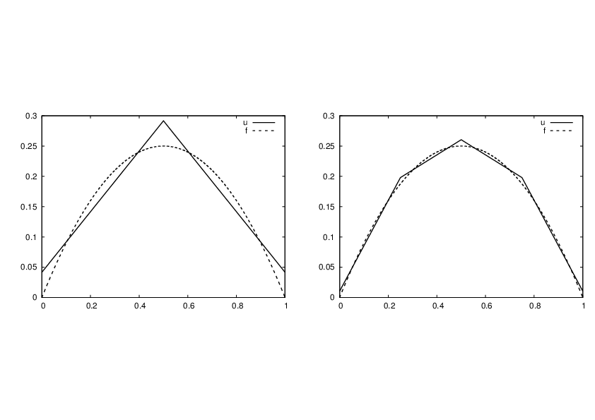
With the aid of the approximate function in the fe_approx1D module we can easily investigate the quality of various finite element approximations to some given functions. Figure Comparison of the finite element approximations: 4 P1 elements with 5 nodes (upper left), 2 P2 elements with 5 nodes (upper right), 8 P1 elements with 9 nodes (lower left), and 4 P2 elements with 9 nodes (lower right) shows how linear and quadratic elements approximates the polynomial \(f(x)=x(1-x)^8\) on \(\Omega =[0,1]\), using equal-sized elements. The results arise from the program
import sympy as sm
from fe_approx1D import approximate
x = sm.Symbol('x')

approximate(f=x*(1-x)**8, symbolic=False, d=1, n_e=4)
approximate(f=x*(1-x)**8, symbolic=False, d=2, n_e=2)
approximate(f=x*(1-x)**8, symbolic=False, d=1, n_e=8)
approximate(f=x*(1-x)**8, symbolic=False, d=2, n_e=4)
The quadratic functions are seen to be better than the linear ones for the same value of \(N\), as we increase \(N\). This observation has some generality: higher degree is not necessarily better on a coarse mesh, but it is as we refined the mesh.
Comparison of the finite element approximations: 4 P1 elements with 5 nodes (upper left), 2 P2 elements with 5 nodes (upper right), 8 P1 elements with 9 nodes (lower left), and 4 P2 elements with 9 nodes (lower right)
Sparse matrix storage and solution
Some of the examples in the preceding section took several minutes to compute, even on small meshes consisting of up to eight elements. The main explanation for slow computations is unsuccessful symbolic integration: sympy may use a lot of energy on integrals like \(\int f(x(X)){\tilde{\varphi}}_r(X)h/2 dx\) before giving up, and the program resorts to numerical integration. Codes that can deal with a large number of basis functions and accept flexible choices of \(f(x)\) should compute all integrals numerically and replace the matrix objects from sympy by the far more efficient array objects from numpy.
A matrix whose majority of entries are zeros, are known as a sparse matrix. We know beforehand that matrices from finite element approximations are sparse. The sparsity should be utilized in software as it dramatically decreases the storage demands and the CPU-time needed to compute the solution of the linear system. This optimization is not critical in 1D problems where modern computers can afford computing with all the zeros in the complete square matrix, but in 2D and especially in 3D, sparse matrices are fundamental for feasible finite element computations.
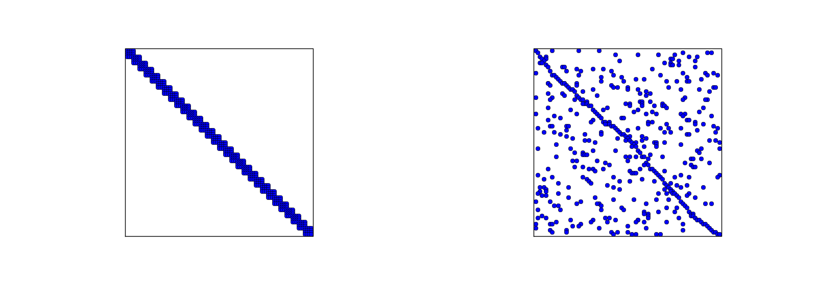
For one-dimensional finite element approximation problems, using a numbering of nodes and elements from left to right over the domain, the assembled coefficient matrix has only a few diagonals different from zero. More precisely, \(2d+1\) diagonals are different from zero. With a different numbering of global nodes, say a random ordering, the diagonal structure is lost, but the number of nonzero elements is unaltered. Figures Matrix sparsity pattern for left-to-right numbering (left) and random numbering (right) of nodes in P1 elements and Matrix sparsity pattern for left-to-right numbering (left) and random numbering (right) of nodes in P3 elements exemplifies sparsity patterns.
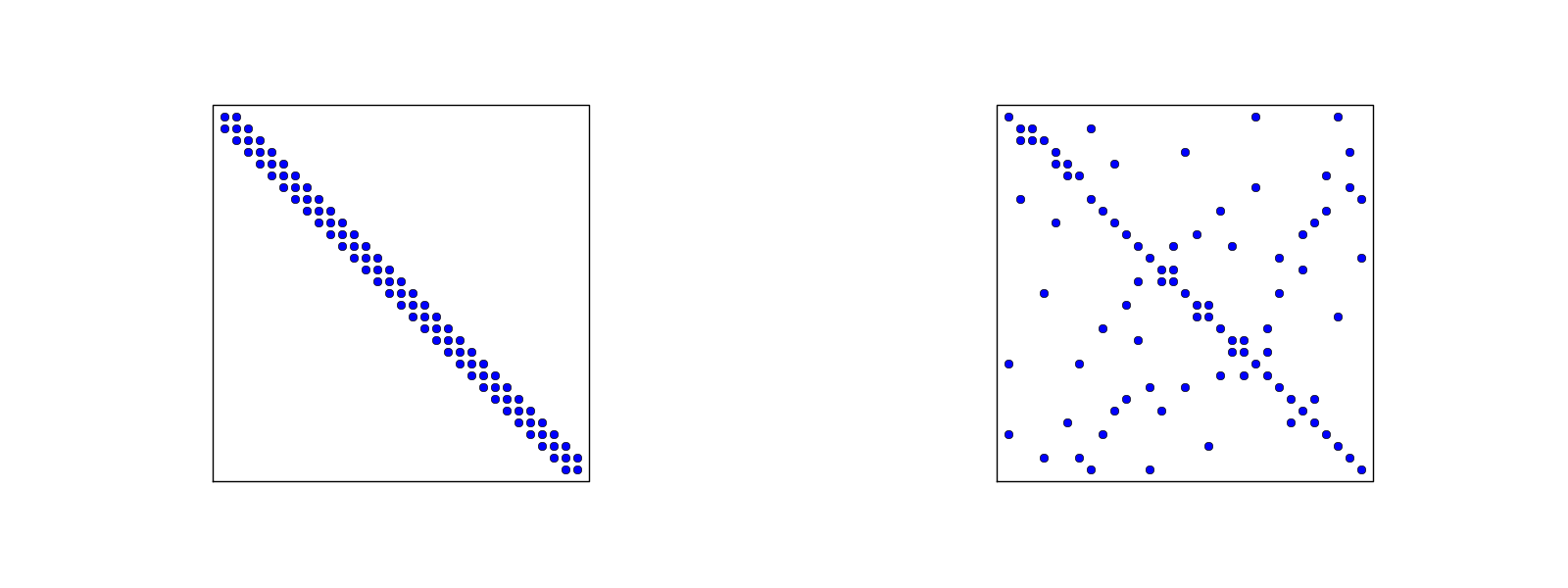
Matrix sparsity pattern for left-to-right numbering (left) and random numbering (right) of nodes in P1 elements
Matrix sparsity pattern for left-to-right numbering (left) and random numbering (right) of nodes in P3 elements
The scipy.sparse library supports creation of sparse matrices and linear system solution.
- scipy.sparse.diags for matrix defined via diagonals
- scipy.sparse.lil_matrix for creation via setting elements
- scipy.sparse.dok_matrix for creation via setting elements
Examples to come....
Comparison of finite element and finite difference approximation
The previous sections on approximating \(f\) by a finite element function \(u\) utilize the projection/Galerkin or least squares approaches to minimize the approximation error. We may, alternatively, use the collocation/interpolation method. Here we shall compare these three approaches with what one does in the finite difference method when representing a given function on a mesh.
Collocation or interpolation
Let \(x_{i}\), \(i=0,\ldots,N\), be the nodes in the mesh. Collocation means
which translates to
but \({\varphi}_j(x_{i})=0\) if \(i\neq j\) so the sum collapses to one term \(c_i{\varphi}_i(x_{i}) = c_i\), and we have the result
That is, \(u\) interpolates \(f\) at the node points (the values coincide at these points, but the variation between the points is dictated by the type of polynomials used in the expansion for \(u\)). The collocation/interpolation approach is obviously much simpler and faster to use than the least squares or projection/Galerkin approach.
Remark. When dealing with approximation of functions via finite elements, all the three methods are in use, while the least squares and collocation methods are used to only a small extend when solving differential equations.
Finite difference approximation of given functions
Approximating a given function \(f(x)\) on a mesh in a finite difference context will typically just sample \(f\) at the grid points. That is, the discrete version of \(f(x)\) is the set of point values \(f(x_i)\), \(i=0,\ldots,N\), where \(x_i\) denotes a mesh point. The collocation/interpolation method above gives exactly the same representation.
How does a finite element Galerkin or least squares approximation differ from this straightforward interpolation of \(f\)? This is the question to be addressed next.
Finite difference interpretation of a finite element approximation
We now limit the scope to P1 elements since this is the element type that gives formulas closest to what one gets from the finite difference method.
The linear system arising from a Galerkin or least squares approximation reads
For P1 elements and a uniform mesh of element length \(h\) we have calculated the matrix with entries \(({\varphi}_i,{\varphi}_j)\) in the section Calculating the linear system. Equation number \(i\) reads
The finite difference counterpart of this equation is just \(u_i=f_i\). (The first and last equation, corresponding to \(i=0\) and \(i=N\) are slightly different, see the section The structure of the coefficient matrix.)
The left-hand side of (27) can be manipulated to equal
Thinking in terms of finite differences, this is nothing but the standard discretization of
or written as
with difference operators.
Before interpreting the approximation procedure as solving a differential equation, we need to work out what the right-hand side is in the context of P1 elements. Since \({\varphi}_i\) is the linear function that is 1 at \(x_{i}\) and zero at all other nodes, only the interval \([x_{i-1},x_{i+1}]\) contributes to the integral on the right-hand side. This integral is naturally split into two parts according to (20):
However, if \(f\) is not known we cannot do much else with this expression. It is clear that many values of \(f\) around \(x_{i}\) contributes to the right-hand side, not just the single point value \(f(x_{i})\) as in the finite difference method.
To proceed with the right-hand side, we turn to numerical integration schemes. Let us say we use the Trapezoidal method for \((f,{\varphi}_i)\), based on the node points \(x_{i}=i h\):
Since \({\varphi}_i\) is zero at all these points, except at \(x_{i}\), the Trapezoidal rule collapses to one term:
for \(i=1,\ldots,N-1\), which is the same result as with collocation/interpolation, and of course the same result as in the finite difference method. For \(i=0\) and \(i=N\) we get contribution from only one element so
Turning to Simpson’s rule with sample points also in the middle of the elements, \(x_i=i h/2\), \(i=0,\ldots,2N\), it reads in general
where \(\tilde h = x_i - x_{i-1}= h/2\) is the spacing between the sample points. We see that the midpoints with odd numbers have the weight \(2h/3\) while the node points with even numbers have the weight \(h/3\). Since \({\varphi}_i=0\) at the even numbers, except for \(x_{2i}=x_{i}\), and \({\varphi}_i=0\) at all the midpoints, on the midpoints and \(4h/3\) on the node points. Since \({\varphi}_i\) vanishes at all the node points, except \(\xi{i}\), and except \(x_{2i-1}=\xi{i}-h/2\) and \(x_{2i+1}=\xi{i}+h/2\), where \({\varphi}_i=1/2\), we get
In a finite difference context we would typically express this formula as
This shows that, with Simpson’s rule, the finite element method operates with the average of \(f\) over three points, while the finite difference method just applies \(f\) at one point. We may interpret this as a “smearing” or smoothing of \(f\) by the finite element method.
We can now summarize our findings. With the approximation of \((f,{\varphi}_i)\) by the Trapezoidal rule, P1 elements give rise to equations that can be expressed as a finite difference discretization of
expressed with operator notation as
As \(h\rightarrow 0\), the extra term proportional to \(u''\) goes to zero, and the two methods are then equal.
With the Simpson’s rule, we may say that we solve
where \(\bar f_i\) means the average \(\frac{1}{3}(f_{i-1/2} + f_i + f_{i+1/2})\).
The extra term \(\frac{h^2}{6} u''\) represents a smoothing: with just this term, we would find u by integrating \(f\) twice and thereby smooth \(f\) considerably. In addition, the finite element representation of \(f\) involves an average, or a smoothing, of \(f\) on the right-hand side of the equation system. If \(f\) is a noisy function, direct interpolation \(u_i=f_i\) may result in a noisy \(u\) too, but with a Galerkin or least squares formulation and P1 elements, we should expect that \(u\) is smoother than \(f\) unless \(h\) is very small.
The interpretation that finite elements tend to smooth the solution is valid in applications far beyond approximation of 1D function.
Making finite elements behave as finite differences
With a simple trick, using numerical integration, we can easily produce the same result \(u_i=f_i\) with the Galerkin or least square formulation with P1 elements. This is useful in many occasions when we deal with more difficult differential equations and want the finite element method to have properties like the finite difference method (solving standard linear wave equations is one primary example).
We have already seen that applying the Trapezoidal rule to the right-hand side \((f,{\varphi}_i)\) simply gives \(f\) sampled at \(x_{i}\). Using the Trapezoidal rule on the matrix entries \(({\varphi}_i,{\varphi}_j)\) involves a sum
but \({\varphi}_i(x_{k})=0\) for all \(k\), except \(k=i\), and \({\varphi}_j(x_{k})=0\) for all \(k\), except \(k=j\). The product \({\varphi}_i{\varphi}_j\) is then different from zero only when sampled at \(x_{i}\) and \(i=j\). The approximation to the integral is then
and zero if \(i\neq j\). This means that we have obtained a diagonal matrix! The first and last diagonal elements, \(({\varphi}_0,{\varphi}_0)\) and \(({\varphi}_N,{\varphi}_N)\) get contribution only from the first and last element, respectively, resulting in the approximate integral value \(h/2\). The corresponding right-hand side also has a factor \(1/2\) for \(i=0\) and \(i=N\). Therefore, the least squares or Galerkin approach with P1 elements and Trapezoidal integration results in
Simpsons’s rule can be used to achieve a similar result for P2 elements, i.e, a diagonal coefficient matrix, but with the previously derived average of \(f\) on the right-hand side.
Elementwise computations (1)
Identical results to those above will arise if we perform elementwise computations. The idea is to use the Trapezoidal rule on the reference element for computing the element matrix and vector. When assembled, the same equations \(c_i=f(x_{i})\) arise. Exercise 16: Use the Trapezoidal rule and P1 elements encourages you to carry out the details.
Terminology
The matrix with entries \(({\varphi}_i,{\varphi}_j)\) typically arises from terms proportional to \(u\) in a differential equation where \(u\) is the unknown function. This matrix is often called the mass matrix, because in the early days of the finite element method, the matrix arose from the mass times acceleration term in Newton’s second law of motion. Making the mass matrix diagonal by, e.g., numerical integration, as demonstrated above, is a widely used technique and is called mass lumping. In time-dependent problems it can enhance the numerical accuracy and computational efficiency of the finite element method. However, there are also examples where mass lumping destroys accuracy.
A generalized element concept
So far, finite element computing has employed the nodes and element lists together with the definition of the basis functions in the reference element. Suppose we want to introduce a piecewise constant approximation with one basis function \({\tilde{\varphi}}_0(x)=1\) in the reference element. Although we could associate the function value with a node in the middle of the elements, there are no nodes at the ends, and the previous code snippets will not work because we cannot find the element boundaries from the nodes list.
Cells, vertices, and degrees of freedom
We now introduce cells as the subdomains \(\Omega^{(e)}\) previously referred as elements. The cell boundaries are denoted as vertices. The reason for this name is that cells are recognized by their vertices in 2D and 3D. Then we define a set of degrees of freedom, which are the quantities we aim to compute. The most common type of degree of freedom is the value of the unknown function \(u\) at some point. For example, we can introduce nodes as before and say the degrees of freedom are the values of \(u\) at the nodes. The basis functions are constructed so that they equal unity for one particular degree of freedom and zero for the rest. This property ensures that when we evaluate \(u=\sum_j c_j{\varphi}_j\) for degree of freedom number \(i\), we get \(u=c_i\). Integrals are performed over cells, usually by mapping the cell of interest to a reference cell.
With the concepts of cells, vertices, and degrees of freedom we increase the decoupling the geometry (cell, vertices) from the space of basis functions. We can associate different sets of basis functions with a cell. In 1D, all cells are intervals, while in 2D we can have cells that are triangles with straight sides, or any polygon, or in fact any two-dimensional geometry. Triangles and quadrilaterals are most common, though. The popular cell types in 3D are tetrahedra and hexahedra.
Extended finite element concept
The concept of a finite element is now
- a reference cell in a local reference coordinate system;
- a set of basis functions \({\tilde{\varphi}}_i\) defined on the cell;
- a set of degrees of freedom that uniquely determine the basis functions such that \({\tilde{\varphi}}_i=1\) for degree of freedom number \(i\) and \({\tilde{\varphi}}_i=0\) for all other degrees of freedom;
- a mapping between local and global degree of freedom numbers;
- a mapping of the reference cell onto to cell in the physical domain.
There must be a geometric description of a cell. This is trivial in 1D since the cell is an interval and is described by the interval limits, here called vertices. If the cell is \(\Omega^{(e)}=[x_L,x_R]\), vertex 0 is \(x_L\) and vertex 1 is \(x_R\). The reference cell in 1D is \([-1,1]\) in the reference coordinate system \(X\).
Our previous P1, P2, etc., elements are defined by introducing \(d+1\) equally spaced nodes in the reference cell and saying that the degrees of freedom are the \(d+1\) function values at these nodes. The basis functions must be 1 at one node and 0 at the others, and the Lagrange polynomials have exactly this property. The nodes can be numbered from left to right with associated degrees of freedom that are numbered in the same way. The degree of freedom mapping becomes what was previously represented by the elements lists. The cell mapping is the same affine mapping (23) as before.
The expansion of \(u\) over one cell is often used. In terms of reference coordinates we have
where the sum is taken over the numbers of the degrees of freedom and \(c_r\) is the value of \(u\) for degree of freedom number \(r\).
Implementation (2)
Implementationwise,
- we replace nodes by vertices;
- we introduce cells such that cell[e][r] gives the mapping from local vertex r in cell e to the global vertex number in vertices;
- we replace elements by dof_map (the contents are the same).
Consider the example from the section Elements and nodes where \(\Omega =[0,1]\) is divided into two cells, \(\Omega^{(0)}=[0,0.4]\) and \(\Omega^{(1)}=[0.4,1]\). The vertices are \([0,0.4,1]\). Local vertex 0 and 1 are \(0\) and \(0.4\) in cell 0 and \(0.4\) and \(1\) in cell 1. A P2 element means that the degrees of freedom are the value of \(u\) at three equally spaced points (nodes) in each cell. The data structures become
vertices = [0, 0.4, 1]
cells = [[0, 1], [1, 2]]
dof_map = [[0, 1, 2], [1, 2, 3]]
If we would approximate \(f\) by piecewise constants, we simply introduce one point or node in an element, preferably \(X=0\), and choose \({\tilde{\varphi}}_0(X)=1\). Only the dof_map is altered:
dof_map = [[0], [1], [2]]
We use the cells and vertices lists to retrieve information on the geometry of a cell, while dof_map is used in the assembly of element matrices and vectors. For example, the Omega_e variable (representing the cell interval) in previous code snippets must now be computed as
Omega_e = [vertices[cells[e][0], vertices[cells[e][1]]
The assembly is done by
A[dof_map[e][r], dof_map[e][s]] += A_e[r,s]
b[dof_map[e][r]] += b_e[r]
We will hereafter work with cells, vertices, and dof_map.
Cubic Hermite polynomials
The finite elements considered so far represent \(u\) as piecewise polynomials with discontinuous derivatives at the cell boundaries. Sometimes it is desired to have continuous derivatives. A primary examples is the solution of differential equations with fourth-order derivatives where standard finite element formulations lead to a need for basis functions with continuous first-order derivatives. The most common type of such basis functions in 1D is the cubic Hermite polynomials.
There are ready-made formulas for the cubic Hermite polynomials, but it is instructive to apply the principles for constructing basis functions in detail. Given a reference cell \([-1,1]\), we seek cubic polynomials with the values of the function and its first-order derivative at \(X=-1\) and \(X=1\) as the four degrees of freedom. Let us number the degrees of freedom as
- 0: value of function at \(X=-1\)
- 1: value of first derivative at \(X=-1\)
- 2: value of function at \(X=1\)
- 3: value of first derivative at \(X=1\)
By having the derivatives as unknowns, we ensure that the derivative of a basis function in two neighboring elements is the same at the node points.
The four basis functions can be written in a general form
with four coefficients \(C_{i,j}\), \(j=0,1,2,3\), to be determined for each \(i\). The constraints that basis function number \(i\) must be 1 for degree of freedom number \(i\) and zero for the other three degrees of freedom, gives four equations to determine \(C_{i,j}\) for each \(i\). In mathematical detail,
These four \(4\times 4\) linear equations can be solved, yielding these formulas for the cubic basis functions:
Remaining tasks:
- Global numbering of the dofs
- dof_map
- 4x4 element matrix
Numerical integration (1)
Finite element codes usually apply numerical approximations to integrals. Since the integrands in the coefficient matrix often are (lower-order) polynomials, integration rules that can integrate polynomials exactly are popular.
The numerical integration rules can be expressed in a common form,
where \(\bar X_j\) are integration points and \(w_j\) are integration weights, \(j=0,\ldots,M\). Different rules correspond to different choices of points and weights.
The very simplest method is the Midpoint rule,
which integrates linear functions exactly.
Newton-Cotes rules
The Newton-Cotes rules are based on a fixed uniform distribution of the points. The first two formulas in this family is the well-known Trapezoidal rule,
and Simpson’s rule,
where
Newton-Cotes rules up to five points is supported in the module file numint.py.
For higher accuracy one can divide the reference cell into a set of subintervals and use the rules above on each subinterval. This approach results in composite rules, well-known from basic introductions to numerical integration of \(\int_{a}^{b}f(x)dx\).
Gauss-Legendre rules with optimized points
All these rules apply equally spaced points. More accurate rules, for a given \(M\), arise if the location of the points are optimized for polynomial integrands. The Gauss-Legendre rules (also known as Gauss-Legendre quadrature or Gaussian quadrature) constitute one such class of integration methods. Two widely applied Gauss-Legendre rules in this family have the choice
These rules integrate 3rd and 5th degree polynomials exactly. In general, an \(M\)-point Gauss-Legendre rule integrates a polynomial of degree \(2M+1\) exactly. The code numint.py contains a large collection of Gauss-Legendre rules.
Approximation of functions in 2D
All the concepts and algorithms developed for approximation of 1D functions \(f(x)\) can readily be extended to 2D functions \(f(x,y)\) and 3D functions \(f(x,y,z)\). Basically, the extensions consists of defining basis functions \({\varphi}_i(x,y)\) or \({\varphi}_i(x,y,z)\) over some domain \(\Omega\), and for the least squares and Galerkin methods, the integration is done over \(\Omega\).
Global basis functions (1)
An example will demonstrate the necessary extensions to use global basis functions and the least squares, Galerkin/projection, or interpolation/collocation methods in 2D. The former two lead to linear systems
where the inner product of two functions \(f(x,y)\) and \(g(x,y)\) is defined completely analogously to the 1D case (12):
Constructing 2D basis functions from 1D functions
One straightforward way to construct a basis in 2D is to combine 1D basis functions. Say we have the 1D basis
We can now form 2D basis functions as products of 1D basis functions: \(\hat{\varphi}_p(x)\hat{\varphi}_q(y)\) for \(p=0,\ldots,N_x\) and \(q=0,\ldots,N_y\). We can either work with double indices, \({\varphi}_{p,q}(x,y) = \hat{\varphi}_p(x)\hat{\varphi}_q(y)\), and write
or we may transform the double index \((p,q)\) to a single index \(i\), using \(i=p N_y + q\) or \(i=q N_x + p\).
Suppose we choose \(\hat{\varphi}_p(x)=x^p\), and try an approximation with \(N_x=N_y=1\):
Using a mapping to one index like \(i=q N_x + p\), we get
Hand calculations
With the specific choice \(f(x,y) = (1+x^2)(1+2y^2)\) on \(\Omega = [0,L_x]\times [0,L_y]\), we can perform actual calculations:
The right-hand side vector has the entries
There is a general pattern in these calculations that we can explore. An arbitrary matrix entry has the formula
where
are matrix entries for one-dimensional approximations. Moreover, \(i=q N_y+q\) and \(j=s N_y+r\).
With \(\hat{\varphi}_p(x)=x^p\) we have
and
for \(p,r=0,\ldots,N_x\) and \(q,s=0,\ldots,N_y\).
Corresponding reasoning for the right-hand side leads to
Choosing \(L_x=L_y=2\), we have
Figure Approximation of a 2D quadratic function (left) by a 2D bilinear function (right) using the Galerkin or least squares method illustrates the result.
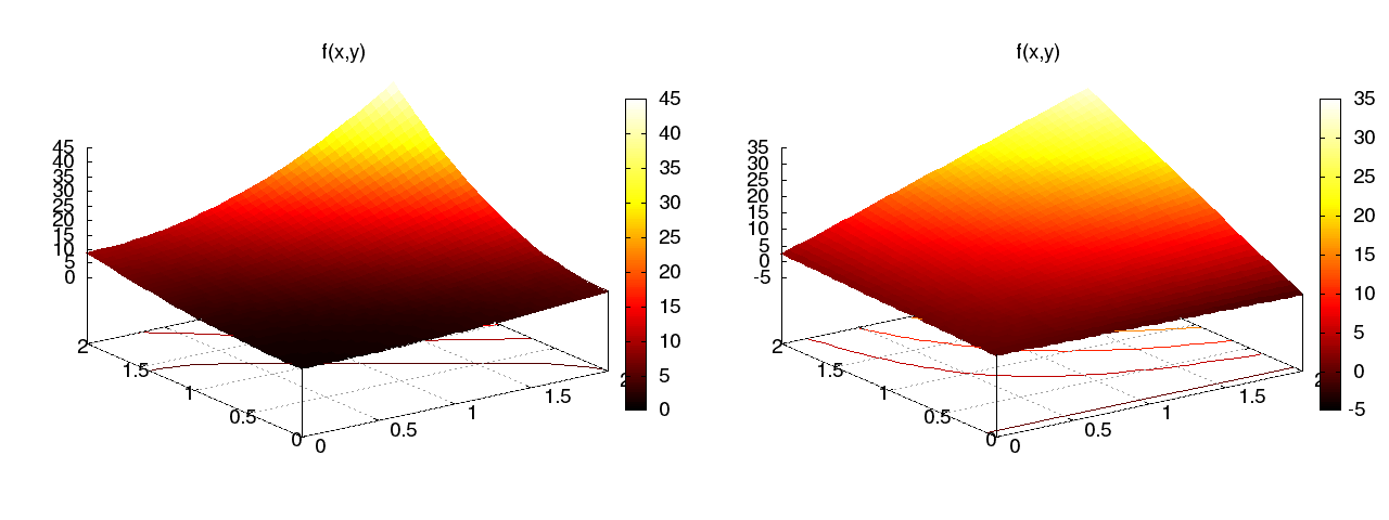
Approximation of a 2D quadratic function (left) by a 2D bilinear function (right) using the Galerkin or least squares method
Implementation (3)
The least_squares function from the section Orthogonal basis functions and/or the file approx1D.py can with very small modifications solve 2D approximation problems. First, let Omega now be a list of the intervals in \(x\) and \(y\) direction. For example, \(\Omega = [0,L_x]\times [0,L_y]\) can be represented by Omega = [[0, L_x], [0, L_y]].
Second, the symbolic integration must be extended to 2D:
import sympy as sm

integrand = phi[i]*phi[j]
I = sm.integrate(integrand,
                 (x, Omega[0][0], Omega[0][1]),
                 (y, Omega[1][0], Omega[1][1]))
provided integrand is an expression involving the sympy symbols x and y. The 2D version of numerical integration becomes
if isinstance(I, sm.Integral):
    integrand = sm.lambdify([x,y], integrand)
    I = sm.mpmath.quad(integrand,
                       [Omega[0][0], Omega[0][1]],
                       [Omega[1][0], Omega[1][1]])
The right-hand side integrals are modified in a similar way.
Third, we must construct a list of 2D basis functions, e.g.,
def taylor(x, y, Nx, Ny):
    return [x**i*y**j for i in range(Nx+1) for j in range(Ny+1)]

def sines(x, y, Nx, Ny):
    return [sm.sin(sm.pi*(i+1)*x)*sm.sin(sm.pi*(j+1)*y)
            for i in range(Nx+1) for j in range(Ny+1)]
The complete code appears in approx2D.py.
The previous hand calculation where a quadratic \(f\) was approximated by a bilinear function can be computed symbolically by
>>> f = (1+x**2)*(1+2*y**2)
>>> phi = taylor(x, y, 1, 1)
>>> Omega = [[0, 2], [0, 2]]
>>> u = least_squares(f, phi, Omega)
>>> print u
8*x*y - 2*x/3 + 4*y/3 - 1/9
>>> print sm.expand(f)
2*x**2*y**2 + x**2 + 2*y**2 + 1
We may continue with adding higher powers to the basis and check that with \(N_x\geq 2\) and \(N_y\geq 2\) we recover the exact function \(f\):
>>> phi = taylor(x, y, 2, 2)
>>> u = least_squares(f, phi, Omega)
>>> print u
2*x**2*y**2 + x**2 + 2*y**2 + 1
>>> print u-f
0
Finite elements in 2D and 3D
Finite element approximation is particularly powerful in 2D and 3D because the method can handle a geometrically complex domain \(\Omega\) with ease. The principal idea is, as in 1D, to divide the domain into cells use polynomials for approximating a function over a cell. Two popular cell shapes are triangles and the quadrilaterals. Figures Examples on 2D P1 elements, Examples on 2D P1 elements in a deformed geometry, and Examples on 2D Q1 elements provide examples. P1 elements means linear functions (\(a_0 + a_1x + a_2y\)) over triangles, while Q1 elements have bilinear functions (\(a_0 + a_1x + a_2y + a_3xy\)) over rectangular cells. Higher-order elements can easily be defined.
Examples on 2D P1 elements
Examples on 2D P1 elements in a deformed geometry
Examples on 2D Q1 elements
Basis functions over triangles in the physical domain
Cells with triangular shape will be in main focus here. With the P1 triangular element, \(u\) is a linear function over each cell, with discontinuous derivatives at the cell boundaries, as depicted in Figure Example on piecewise linear 2D functions defined on triangles.
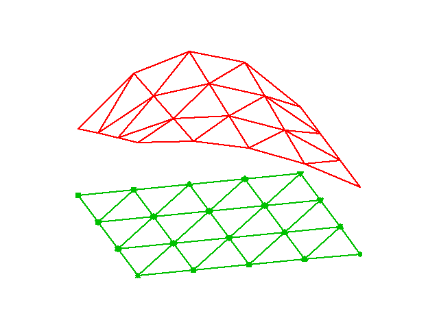
Example on piecewise linear 2D functions defined on triangles
We give the vertices of the cells global and local numbers as in 1D. The degrees of freedom in the P1 element are the function values at a set of nodes, which are the three vertices. The basis function \({\varphi}_i(x,y)\) is then 1 at the vertex with global vertex number \(i\) and zero at all other vertices. On an element, the three degrees of freedom uniquely determine the linear basis functions in that element, as usual. The global \({\varphi}_i(x,y)\) function is then a combination of the linear functions (planar surfaces) over all the neighboring cells that have vertex number \(i\) in common. Figure Example on a piecewise linear 2D basis function over a patch of triangles tries to illustrate the shape of such a “pyramid”-like function.
Example on a piecewise linear 2D basis function over a patch of triangles
Element matrices and vectors
As in 1D, we split the integral over \(\Omega\) into a sum of integrals over cells. Also as in 1D, \({\varphi}_i\) overlaps \({\varphi}_j\) (i.e., \({\varphi}_i{\varphi}_j\neq 0\)) if and only if \(i\) and \(j\) are vertices in the same cell. Therefore, the integral of \({\varphi}_i{\varphi}_j\) over an element is nonzero only when \(i\) and \(j\) run over the vertex numbers in the element. These nonzero contributions to the coefficient matrix are, as in 1D, collected in an element matrix. The size of the element matrix becomes \(3\times 3\) since there are three degrees of freedom that \(i\) and \(j\) run over. Again, as in 1D, we number the local vertices in a cell, starting at 0, and add the entries in the element matrix into the global system matrix, exactly as in 1D. All details and code appear below.
Basis functions over triangles in the reference cell
As in 1D, we can define the basis functions and the degrees of freedom in a reference cell and then use a mapping from the reference coordinate system to the physical coordinate system. We also have a mapping of local degrees of freedom numbers to global degrees of freedom numbers. .. (dof_map).
The reference cell in an \((X,Y)\) coordinate system has vertices \((0,0)\), \((1,0)\), and \((0,1)\), corresponding to local vertex numbers 0, 1, and 2, respectively. The P1 element has linear functions \({\tilde{\varphi}}_r(X,Y)\) as basis functions, \(r=0,1,2\). Since a linear function \({\tilde{\varphi}}_r(X,Y)\) in 2D is on the form \(C_{r,0} + C_{r,1}X + C_{r,2}Y\), and hence has three parameters \(C_{r,0}\), \(C_{r,1}\), and \(C_{r,2}\), we need three degrees of freedom. These are in general taken as the function values at a set of nodes. For the P1 element the set of nodes is the three vertices. Figure 2D P1 element displays the geometry of the element and the location of the nodes.

2D P1 element
Requiring \({\tilde{\varphi}}_r=1\) at node number \(r\) and \({\tilde{\varphi}}_r=0\) at the two other nodes, gives three linear equations to determine \(C_{r,0}\), \(C_{r,1}\), and \(C_{r,2}\). The result is
Higher-order approximations are obtained by increasing the polynomial order, adding additional nodes, and letting the degrees of freedom be function values at the nodes. Figure 2D P2 element shows the location of the six nodes in the P2 element.

2D P2 element
A polynomial of degree \(p\) in \(X\) and \(Y\) has \(n_p=(p+1)(p+2)/2\) terms and hence needs \(n_p\) nodes. The values at the nodes constitute \(n_p\) degrees of freedom. The location of the nodes for \({\tilde{\varphi}}_r\) up to degree 6 is displayed in Figure 2D P1, P2, P3, P4, P5, and P6 elements.
2D P1, P2, P3, P4, P5, and P6 elements
The generalization to 3D is straightforward: the reference element is a tetrahedron with vertices \((0,0,0)\), \((1,0,0)\), \((0,1,0)\), and \((0,0,1)\) in a \(X,Y,Z\) reference coordinate system. The P1 element has its degrees of freedom as four nodes, which are the four vertices, see Figure P1 elements in 1D, 2D, and 3D. The P2 element adds additional nodes along the edges of the cell, yielding a total of 10 nodes and degrees of freedom, see Figure P2 elements in 1D, 2D, and 3D.
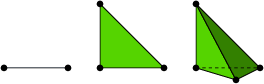
P1 elements in 1D, 2D, and 3D
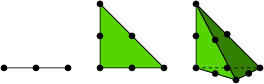
P2 elements in 1D, 2D, and 3D
The interval in 1D, the triangle in 2D, the tetrahedron in 3D, and its generalizations to higher space dimensions are known as simplex cells (the geometry) or simplex elements (the geometry, basis functions, degrees of freedom, etc.). The plural forms simplices and simplexes are also a much used shorter terms when referring to this type of cells or elements. The side of a simplex is called a face, while the tetrahedron also has edges.
Acknowledgment. Figures 2D P1 element to P2 elements in 1D, 2D, and 3D are created by Anders Logg and taken from the FEniCS book: Automated Solution of Differential Equations by the Finite Element Method, edited by A. Logg, K.-A. Mardal, and G. N. Wells, published by Springer, 2012.
Affine mapping of the reference cell
Let \({\tilde{\varphi}}_r^{(1)}\) denote the basis functions associated with the P1 element in 1D, 2D, or 3D, and let \(\pmb{x}_{q(e,r)}\) be the physical coordinates of local vertex number \(r\) in cell \(e\). Furthermore, let \(\pmb{X}\) be a point in the reference coordinate system corresponding to the point \(\pmb{x}\) in the physical coordinate system. The affine mapping of any \(\pmb{X}\) onto \(\pmb{x}\) is then defined by
where \(r\) runs over the local vertex numbers in the cell. The affine mapping maps the straight or planar faces of the reference cell onto straight or planar faces in the physical coordinate system. The mapping can be used for both P1 and higher-order elements.

Affine mapping of a P1 element
Isoparametric mapping of the reference cell
Instead of using the P1 basis functions in the mapping (29), we may use the basis functions of the actual element:
where \(r\) runs over all nodes, i.e., all points associated with the degrees of freedom. This is called an isoparametric mapping. For P1 elements it is identical to the affine mapping (29), but for higher-order elements the mapping of the straight or planar faces of the reference cell will result in a curved face in the physical coordinate system. For example, when we use the basis functions of the triangular P2 element in 2D in (30), the straight faces of the reference triangle are mapped onto curved faces of parabolic shape in the physical coordinate system, see Figure Isoparametric mapping of a P2 element.

Isoparametric mapping of a P2 element
From (29) or (30) it is easy to realize that the vertices are correctly mapped. Consider a vertex with local number \(s\). Then \({\tilde{\varphi}}_s=1\) at this vertex and zero at the others. This means that only one term in the sum is nonzero and \(\pmb{x}=\pmb{x}_{q(e,s)}\), which is the coordinate of this vertex in the global coordinate system.
Computing integrals
Let \(\tilde\Omega^r\) denote the reference cell and \(\Omega^{(e)}\) the cell in the physical coordinate system. The transformation of the integral from the physical to the reference coordinate system reads
where \(d\pmb{x} = dx dy\) in 2D and \(d\pmb{x} = dx dy dz\) in 3D, with a similar definition of \(d\pmb{X}\). The quantity \(\det J\) is the determinant of the Jacobian of the mapping \(\pmb{x}(\pmb{X})\). In 2D,
With the affine mapping (29), \(\det J=2\Delta\), where \(\Delta\) is the area or volume of the cell in the physical coordinate system.
Remark. Observe that finite elements in 2D and 3D builds on the same ideas and concepts as in 1D, but there is simply more to compute because the specific mathematical formulas in 2D and 3D are more complicated.
Exercises (1)
Exercise 1: Linear algebra refresher I
Look up the topic of vector space in your favorite linear algebra book or search for the term at Wikipedia. Prove that vectors in the plane \((a,b)\) form a vector space by showing that all the axioms of a vector space are satisfied. Similarly, prove that all linear functions of the form \(ax+b\) constitute a vector space, \(a,b\in\mathbb{R}\).
On the contrary, show that all quadratic functions of the form \(1 + ax^2 + bx\) do not constitute a vector space. Filename: linalg1.
Exercise 2: Linear algebra refresher II
As an extension of Exercise 1: Linear algebra refresher I, check out the topic of inner product spaces. Suggest a possible inner product for the space of all linear functions of the form \(ax+b\), \(a,b\in\mathbb{R}\). Show that this inner product satisfies the general requirements of an inner product in a vector space. Filename: linalg2.
Exercise 3: Approximate a three-dimensional vector in a plane
Given \(\pmb{f} = (1,1,1)\) in \(\mathbb{R}^3\), find the best approximation vector \(\pmb{u}\) in the plane spanned by the unit vectors \((1,0)\) and \((0,1)\). Repeat the calculations using the vectors \((2,1)\) and \((1,2)\). Filename: vec111_approx.
Exercise 4: Approximate the sine function by power functions
Let \(V\) be a function space with basis functions \(x^{2i+1}\), \(i=0,1,\ldots,N\). Find the best approximation to \(f(x)=\sin(x)\) among all functions in \(V\), using \(N=8\) for a domain that includes more and more half-periods of the sine function: \(\Omega = [0, k\pi/2]\), \(k=2,3,\ldots,12\). How does a Taylor series of \(\sin(x)\) around \(x\) up to degree 9 behave for the largest domain?
Hint. One can make a loop over \(k\) and call the least_squares and comparison_plot from the approx1D module. Filename: sin_powers.py.
Exercise 5: Approximate a steep function by sines
Find the best approximation of \(f(x) = \tanh (s(x-\pi))\) on \([0, 2\pi]\) in the space \(V\) with basis \({\varphi}_i(x) = sin((2i+1)x)\), \(i=0,\ldots,N\). Make a movie showing how \(u=\sum_{j=0}^Nc_j{\varphi}_j(x)\) approximates \(f(x)\) as \(N\) grows. Choose \(s\) such that \(f\) is steep (\(s=20\) may be appropriate).
Hint. One may naively call the least_squares_orth and comparison_plot from the approx1D module in a loop and extend the basis with one new element in each pass. This approach implies a lot of recomputations. A more efficient strategy is to let least_squares_orth compute with only one basis function at a time and accumulate the corresponding u in the total solution. Filename: tanh_sines_approx1.py.
Exercise 6: Fourier series as a least squares approximation
Given a function \(f(x)\) on an interval \([0,L]\), find the formula for the coefficients of the Fourier series of \(f\):
Let an infinite-dimensional vector space \(V\) have the basis functions \(\cos j\frac{\pi x}{L}\) for \(j=0,1,\dots,\infty\) and \(\sin j\frac{\pi x}{L}\) for \(j=1,\dots,\infty\). Show that the least squares approximation method from the section Approximation of functions leads to a linear system whose solution coincides with the standard formulas for the coefficients in a Fourier series of \(f(x)\) (see also the section Fourier series). You may choose
for \(i=0,1,\ldots,N\rightarrow\infty\).
Choose \(f(x) = \tanh(s(x-\frac{1}{2}))\) on \(\Omega=[0,1]\), which is a smooth function, but with considerable steepness around \(x=1/2\) as \(s\) grows in size. Calculate the coefficients in the Fourier expansion by solving the linear system, arising from the least squares or Galerkin methods, by hand. Plot some truncated versions of the series together with \(f(x)\) to show how the series expansion converges for \(s=10\) and \(s=100\). Filename: Fourier_approx.py.
Exercise 7: Approximate a steep function by Lagrange polynomials
Use interpolation/collocation with uniformly distributed points and Chebychev nodes to approximate
by Lagrange polynomials for \(s=10,100\) and \(N=3,6,9,11\). Make separate plots of the approximation for each combination of \(s\), point type (Chebyshev or uniform), and \(N\). Filename: tanh_Lagrange.py.
Exercise 8: Define finite element meshes
Consider a domain \(\Omega =[0,2]\) divided into the three elements \([0,1]\), \([1,1.2]\), and \([1.2,2]\), with two nodes in each element (P1 elements). Set up the list of coordinates and nodes (nodes) and the numbers of the nodes that belong to each element (elements) in two cases: 1) nodes and elements numbered from left to right, and 2) nodes and elements numbered from right to left.
Thereafter, subdivide the element \([1.2,2]\) into two new equal-sized elements. Add the new node and the two new elements to the data structures created above, and try to minimize the modifications. Filename: fe_numberings.py..
Exercise 9: Construct matrix sparsity patterns
Exercise 8: Define finite element meshes describes a element mesh with a total of five elements, but with two different element and node orderings. For each of the two orderings, make a \(5\times 5\) matrix and fill in the entries that will be nonzero.
Hint. A matrix entry \((i,j)\) is nonzero if \(i\) and \(j\) are nodes in the same element. Filename: fe_sparsity_pattern.pdf.
Exercise 10: Perform symbolic finite element computations
Find formulas for the coefficient matrix and right-hand side when approximating \(f(x) = sin (x)\) on \(\Omega=[0, \pi]\) by two P1 elements of size \(\pi/2\). Solve the system and compare \(u(\pi/2\) with the exact value 1.
Filename: sin_approx_P1.py.
Exercise 11: Approximate a steep function by P1 and P2 elements
Given
use the Galerkin or least squares method with finite elements to find an approximate function \(u(x)\). Choose \(s=40\) and try \(n_e=4,8,16\) P1 elements and \(n_e=2,4,8\) P2 elements. Integrate \(f{\varphi}_i\) numerically. Filename: tanh_fe_P1P2_approx.py.
Exercise 12: Approximate a \(\tanh\) function by P3 and P4 elements
Solve fem:approx:exer:tanh using \(n_e=1,2,4\) P3 and P4 elements. How will a collocation/interpolation method work in this case with the same number of nodes? Filename: tanh_fe_P3P4_approx.py.
Exercise 13: Investigate the approximation errors in finite elements
A fundamental question is how accurate the finite element approximation is in terms of the cell length \(h\) and the degree \(d\) of the basis functions. We can investigate this empirically by choosing an \(f\) function, say \(f(x) = A\sin (\omega x)\) on \(\Omega=[0, 2\pi/\omega]\), and compute the approximation error for a series of \(h\) and \(d\) values. The theory predicts that the error should behave as \(h^{d+1}\). Use experiments to verify this asymptotic behavior (i.e., for small enough \(h\)). Filename: Asinwt_interpolation_error.py.
Exercise 14: Approximate a step function by finite elements
Approximate the step function
by 2, 4, and 8 P1 and P2 elements. Compare approximations visually.
Hint. This \(f\) can also be expressed in terms of the Heaviside function \(H(x)\): \(f(x) = H(x-{1/2})\). Therefore, \(f\) can be defined by f = sm.Heaviside(x - sm.Rational(1,2)), making the approximate function in the fe_approx1D.py module an obvious candidate to solve the problem. However, sympy does not handle symbolic integration with this particular integrand, and the approximate function faces a problem when converting f to a Python function (for plotting) since Heaviside is not an available function in numpy. It is better to make special-purpose code for this case or perform all calculations by hand. Filename: Heaviside_approx_P1P2.py..
Exercise 15: 2D approximation with orthogonal functions
Assume we have basis functions \({\varphi}_i(x,y)\) in 2D that are orthogonal such that \(({\varphi}_i,{\varphi}_j)=0\) when \(i\neq j\). The function least_squares in the file approx2D.py will then spend much time on computing off-diagonal terms in the coefficient matrix that we know are zero. To speed up the computations, make a version least_squares_orth that utilizes the orthogonality among the basis functions. Apply the function to approximate
on \(\Omega = [0,1]\times [0,1]\) via basis functions
Hint. Get ideas from the function least_squares_orth in the section Orthogonal basis functions and file approx1D.py. Filename: approx2D_lsorth_sin.py.
Exercise 16: Use the Trapezoidal rule and P1 elements
Consider approximation of some \(f(x)\) on an interval \(\Omega\) using the least squares or Galerkin methods with P1 elements. Derive the element matrix and vector using the Trapezoidal rule (28) for calculating integrals on the reference element. Assemble the contributions, assuming a uniform cell partitioning, and show that the resulting linear system has the form \(c_i=f(x_{i})\) for \(i=0,\ldots,N\).
Filename: fe_trapez.pdf.
Basic principles for approximating differential equations
The finite element method is a very flexible approach for solving partial differential equations. Its two most attractive features are the ease of handling domains of complex shape in two and three dimensions and the ease of constructing higher-order discretization methods. The finite element method is usually applied for discretization in space, and therefore spatial problems will be our focus in the coming sections. Extensions to time-dependent problems may, for instance, use finite difference approximations in time.
Before studying how finite element methods are used to tackle differential equation, we first look at how global basis functions and the least squares, Galerkin, and collocation principles can be used to solve differential equations.
Differential equation models
Let us consider an abstract differential equation for a function \(u(x)\) of one variable, written as
Here are a few examples on possible choices of \({\cal L}(u)\), of increasing complexity:
Both \(a(x)\) and \(f(x)\) are considered as specified functions, while \(\alpha\) is a prescribed parameter. Differential equations corresponding to (?)-(?) arise in diffusion phenomena, such as steady transport of heat in solids and flow of viscous fluids between flat plates. The form (?) arises when transient diffusion or wave phenomenon are discretized in time by finite differences. The equation (?) appear in chemical models when diffusion of a substance is combined with chemical reactions. Also in biology, (?) plays an important role, both for spreading of species and in models involving generation and propagation of electrical signals.
Let \(\Omega =[0,L]\) be the domain in one space dimension. In addition to the differential equation, \(u\) must fulfill boundary conditions at the boundaries of the domain, \(x=0\) and \(x=L\). When \({\cal L}\) contains up to second-order derivatives, as in the examples above, \(m=1\), we need one boundary condition at each of the (two) boundary points, here abstractly specified as
There are three common choices of boundary conditions:
Here, \(g\) and \(a\) are specified quantities.
From now on we shall use \(u_{\small\mbox{e}}(x)\) as symbol for the exact solution, fulfilling
while \(u(x)\) denotes an approximate solution of the differential equation. We must immediately remark that in the literature about the finite element method, is common to use \(u\) as the exact solution and \(u_h\) as the approximate solution, where \(h\) is a discretization parameter. However, the vast part of the present text is about the approximate solutions, and having a subscript \(h\) attached all the time is cumbersome. Of equal importance is the close correspondence between implementation and mathematics that we strive to achieve in this book: when it is natural to use u and not u_h in code, we let the mathematical notation be dictated by the code’s preferred notation. After all, it is the powerful computer implementations of the finite element method that justifies studying the mathematical formulation and aspects of the method.
A common model problem used much in the forthcoming examples is
The specific choice of \(f(x)=2\) gives the solution
A closely related problem with a different boundary condition at \(x=0\) reads
A third variant has a variable coefficient,
Residual-minimizing principles
The fundamental idea is to seek an approximate solution \(u\) in some space \(V\) with basis
which means that \(u\) can always be expressed as
for some unknown coefficients \(c_0,\ldots,c_N\). (Later, in the section Boundary conditions: specified value, we will see that if we specify boundary values of \(u\) different from zero, we must look for an approximate solution \(u(x) = B(x) + \sum_{j=0}^N c_j{\varphi}_j(x)\), where \(\sum_{j}c_j{\varphi}_j\in V\) and \(B(x)\) is some function for incorporating the right boundary values. Because of \(B(x)\), \(u\) will not necessarily lie in \(V\). This modification does not imply any difficulties.) As in the section Approximation of functions, we need principles for deriving \(N+1\) equations to determine the \(N+1\) unknowns \(c_0,\ldots,c_N\). A key idea of the section Approximation of functions was to minimize the approximation error \(e=u-f\). That principle is not so useful here since the approximation error \(e=u_{\small\mbox{e}} - u\) is unknown to us when \(u_{\small\mbox{e}}\) is unknown. The only general indicator we have on the quality of the approximate solution is to what degree \(u\) fulfills the differential equation. Inserting \(u=\sum_j c_j {\varphi}_j\) into \({\cal L}(u)\) reveals that the result is not zero, because \(u\) is only likely to equal \(u_{\small\mbox{e}}\). The nonzero result,
is called the residual and measures the error in fulfilling the governing equation. Various principles for determining \(c_0,\ldots,c_N\) try to minimize \(R\) in some sense. Note that \(R\) varies with \(x\) and the \(c_0,\ldots,c_N\) parameters. We may write this dependence explicitly as
The least squares method (4)
The least-squares method aims to find \(c_0,\ldots,c_N\) so that the integrated square of the residual,
is minimized. By introducing an inner product of two functions \(f\) and \(g\) on \(\Omega\) as
the least-squares method can be defined as
Differentiating with respect to the free parameters \(c_0,\ldots,c_N\) gives the \(N+1\) equations
The Galerkin method (1)
The least-squares principle is equivalent to demanding the error to be orthogonal to the space \(V\) when approximating a function \(f\) by \(u\in V\). With a differential equation we do not know the true error so we must instead require the residual \(R\) to be orthogonal to \(V\). This idea implies seeking \(c_0,\ldots,c_N\) such that
This is the Galerkin method for differential equations. As shown in (9) and (10), this statement is equivalent to \(R\) being orthogonal to the \(N+1\) basis functions only:
resulting in \(N+1\) equations for determining \(c_0,\ldots,c_N\).
The Method of Weighted Residuals
A generalization of the Galerkin method is to demand that \(R\) is orthogonal to some space \(W\), but not necessarily the same space as \(V\) where we seek the unknown function. This generalization is naturally called the method of weighted residuals:
If \(\{w_0,\ldots,w_N\}\) is a basis for \(W\), we can equivalently express the method of weighted residuals as
The result is \(N+1\) equations for \(c_0,\ldots,c_N\).
The least-squares method can also be viewed as a weighted residual method with \(w_i = \partial R/\partial c_i\).
Variational Formulation
Formulations like (38) (or (39)) and (36) (or (37)) are known as variational formulations. These equations are in this text primarily used for a numerical approximation \(u\in V\), where \(V\) is a finite-dimensional space with dimension \(N+1\). However, we may also let \(V\) be an infinite-dimensional space containing the exact solution \(u_{\small\mbox{e}}(x)\) such that also \(u_{\small\mbox{e}}\) fulfills a variational formulation. The variational formulation is in that case a mathematical way of stating the problem and acts as an alternative to the usual formulation of a differential equation with initial and/or boundary conditions.
Test and Trial Functions
In the context of the Galerkin method and the method of weighted residuals it is common to use the name trial function for the approximate \(u = \sum_j c_j {\varphi}_j\). .. Sometimes the functions that spans the space where \(u\) lies are also called
The space containing the trial function is known as the trial space. The function \(v\) entering the orthogonality requirement in the Galerkin method and the method of weighted residuals is called test function, and so are the \({\varphi}_i\) or \(w_i\) functions that are used as weights in the inner products with the residual. The space where the test functions comes from is naturally called the test space.
We see that in the method of weighted residuals the test and trial spaces are different and so are the test and trial functions. In the Galerkin method the test and trial spaces are the same (so far). Later in the section Boundary conditions: specified value we shall see that boundary conditions may lead to a difference between the test and trial spaces in the Galerkin method.
Remark. It may be subject to debate whether it is only the form of (38) or (36) after integration by parts, as explained in the section Integration by parts, that qualifies for the term variational formulation. The result after integration by parts is what is obtained after taking the first variation of an optimization problem, see the section Variational problems and optimization of functionals. However, here we use variational formulation as a common term for formulations which, in contrast to the differential equation \(R=0\), instead demand that an average of \(R\) is zero: \((R,v)=0\) for all \(v\) in some space.
The collocation method (1)
The idea of the collocation method is to demand that \(R\) vanishes at \(N+1\) selected points \(x_{0},\ldots,x_{N}\) in \(\Omega\):
The collocation method can also be viewed as a method of weighted residuals with Dirac delta functions as weighting functions. Let \(\delta (x-x_{i})\) be the Dirac delta function centered around \(x=x_{i}\) with the properties that \(\delta (x-x_{i})=0\) for \(x\neq x_{i}\) and
Intuitively, we may think of \(\delta (x-x_{i})\) as a very peak-shaped function around \(x=x_{i}\) with integral 1, roughly visualized in Figure Approximation of delta functions by narrow Gaussian functions. Because of (41), we can let \(w_i=\delta(x-x_{i})\) be weighting functions in the method of weighted residuals, and (39) becomes equivalent to (40).
Approximation of delta functions by narrow Gaussian functions
The subdomain collocation method
The idea of this approach is to demand the integral of \(R\) to vanish over \(N+1\) subdomains \(\Omega_i\) of \(\Omega\):
This statement can also be expressed as a weighted residual method
where \(w_i=1\) for \(x\in\Omega_i\) and \(w_i=0\) otherwise.
Examples on using the principles
Let us now apply global basis functions to illustrate the principles for minimizing \(R\).
The model problem
We consider the differential equation problem
Basis functions
Our choice of basis functions \({\varphi}_i\) for \(V\) is
An important property of these functions is that \({\varphi}_i(0)={\varphi}_i(L)=0\), which means that the boundary conditions on \(u\) are fulfilled:
Another nice property is that the chosen sine functions are orthogonal on \(\Omega\):
provided \(i\) and \(j\) are integers.
The residual
We can readily calculate the following explicit expression for the residual:
The least squares method (5)
The equations (35) in the least squares method require an expression for \(\partial R/\partial c_i\). We have
The governing equations for \(c_0,\ldots,c_N\) are then
which can be rearranged as
This is nothing but a linear system
with
Since the coefficient matrix is diagonal we can easily solve for
With the special choice of \(f(x)=2\) the integral becomes
according to WolframAlpha (use j and not i, which means \(=\sqrt{-1}\), when asking). Hence,
Now, \(1+(-1)^i=0\) for \(i\) odd, so only the coefficients with even index are nonzero. Introducing \(i=2k\) for \(k=0,\ldots,N/2\) to count the relevant indices, we get the solution
The coefficients decay very fast: \(c_2 = c_0/27\), \(c_4=c_0/125\). The solution will therefore be dominated by the first term,
The Galerkin method (2)
The Galerkin principle (36) applied to (42) consists of inserting our special residual (44) in (36)
or
This is the variational formulation, based on the Galerkin principle, of our differential equation. The \(\forall v\in V\) requirement is equivalent to demanding the equation \((u'',v) = -(f,v)\) to be fulfilled for all basis functions \(v={\varphi}_i\), \(i=0,\ldots,N\) (cf. (36) and (37)). This gives
This equation can be rearranged to a form that explicitly shows that we get a linear system for the unknowns \(c_0,\ldots,c_N\):
For the particular choice of the basis functions (43) we get in fact the same linear system as in the least squares method (because \({\varphi}''= -(i+1)^2\pi^2L^{-2}{\varphi}\)).
The collocation method (2)
For the collocation method (40) we need to decide upon a set of \(N+1\) collocation points in \(\Omega\). A simple choice is to use uniformly spaced points: \(x_{i}=i\Delta x\), where \(\Delta x = L/N\) in our case (\(N\geq 1\)). However, these points lead to at least two rows in the matrix consisting of zeros (since \({\varphi}_i(x_{0})=0\) and \({\varphi}_i(x_{N})=0\)), thereby making the matrix singular and non-invertible. This forces us to choose some other collocation points, e.g., random points or points uniformly distributed in the interior of \(\Omega\). Demanding the residual to vanish at these points leads, in our model problem (42), to the equations
which is seen to be a linear system with entries
in the coefficient matrix and entries \(b_i=2\) for the right-hand side (when \(f(x)=2\)).
The special case of \(N=0\) can sometimes be of interest. A natural choice is then the midpoint \(x_{0}=L/2\) of the domain, resulting in \(A_{0,0} = -{\varphi}_0''(x_{0}) = \pi^2L^{-2}\), \(f(x_0)=2\), and hence \(c_0=2L^2/\pi^2\).
Comparison
In the present model problem, with \(f(x)=2\), the exact solution is \(u(x)=x(L-x)\), while for \(N=0\) the Galerkin and least squares method result in \(u(x)=8L^2\pi^{-3}\sin (\pi x/L)\) and the collocation method leads to \(u(x)=2L^2\pi^{-2}\sin (\pi x/L)\). Since all methods fulfill the boundary conditions \(u(0)=u(L)=0\), we expect the largest discrepancy to occur at the midpoint of the domain: \(x=L/2\). The error at the midpoint becomes \(-0.008L^2\) for the Galerkin and least squares method, and \(0.047L^2\) for the collocation method.
Integration by parts
A problem arises if we want to use the finite element functions from the section Finite element basis functions to solve our model problem (42) by the least squares, Galerkin, or collocation methods: the piecewise polynomials \({\varphi}_i(x)\) have discontinuous derivatives at the cell boundaries which makes it problematic to compute \({\varphi}_i''(x)\). This fact actually makes the least squares and collocation methods less suitable for finite element approximation of the unknown function. (By rewriting the equation \(-u''=f\) as a system of two first-order equations, \(u'=v\) and \(-v'=f\), the least squares method can be applied. Also, differentiating discontinuous functions can actually be handled by distribution theory in mathematics.) The Galerkin method and the method of weighted residuals can, however, be applied together with finite element basis functions if we use integration by parts as a means for transforming a second-order derivative to a first-order one.
Consider the model problem (42) and its Galerkin formulation
Using integration by parts in the Galerkin method, we can move a derivative on \(u\) to \(v\):
Usually, one integrates the problem at the stage where the \(u\) and \(v\) functions enter the formulation. Alternatively, but less common, we can integrate by parts in the expressions for the matrix entries:
Integration by parts serves to reduce the order of the derivatives and to make the coefficient matrix symmetric since \(({\varphi}_i',{\varphi}_j') = ({\varphi}_i',{\varphi}_j')\). The symmetry property depends on the type of terms that enter the differential equation. As will be seen later in the section Boundary conditions: specified derivative, integration by parts also provides a method for implementing boundary conditions involving \(u'\).
With the choice (43) of basis functions we see that the “boundary terms” \({\varphi}_i(L){\varphi}_j'(L)\) and \({\varphi}_i(0){\varphi}_j'(0)\) vanish since \({\varphi}_i(0)={\varphi}_i(L)=0\). A boundary term associated with a location at the boundary where we have Dirichlet conditions will always vanish because \({\varphi}_i=0\) at such locations.
Since the variational formulation after integration by parts make weaker demands on the differentiability of \(u\) and the basis functions \({\varphi}_i\), the resulting integral formulation is referred to as a weak form of the differential equation problem. The original variational formulation with second-order derivatives, or the differential equation problem with second-order derivative, is then the strong form, with stronger requirements on the differentiability of the functions.
For differential equations with second-order derivatives, expressed as variational formulations and solved by finite element methods, we will always perform integration by parts to arrive at expressions involving only first-order derivatives.
Boundary function
So far we have assumed zero Dirichlet boundary conditions, typically \(u(0)=u(L)=0\), and we have demanded that \({\varphi}_i(0){\varphi}_i(L)=0\) for \(i=0,\ldots,N\). What about a boundary condition like \(u(L)=D\neq0\)? This condition immediately faces a problem with \(u=\sum_{j=0}^N c_j {\varphi}_j\), because \(u(L)=0\) since all the basis functions vanish at \(x=L\).
A boundary condition of the form \(u(L)=D\) can be implemented by demanding that all \({\varphi}_i(L)=0\), but adding a boundary function \(B(x)\) with the right boundary value, \(B(L)=D\), to the expansion for \(u\):
This \(u\) gets the right value at \(x=L\):
The idea is that for any boundary where \(u\) is known we demand \({\varphi}_i\) to vanish and construct a function \(B(x)\) to attain the boundary value of \(u\). There are no restrictions how \(B(x)\) varies with \(x\) in the interior of the domain, so this variation needs to be constructed in some way.
For example, with \(u(0)=0\) and \(u(L)=D\), we can choose \(B(x)=x D/L\), since \(B(0)=0\) and \(B(L)=D\). The unknown function is then sought on the form
with \({\varphi}_i(0)={\varphi}_i(L)=0\).
The \(B(x)\) function can be chosen in many ways as long as its boundary values are correct. For example, \(B(x)=D(x/L)^p\) for any power \(p\) will work fine in the above example. As another example, consider a domain \(\Omega = [a,b]\) where the boundary conditions are \(u(a)=U_a\) and \(u(b)=U_b\). A class of possible \(B(x)\) functions is
To summarize, the procedure goes as follows. Let \(\partial\Omega_E\) be the part(s) of the boundary \(\partial\Omega\) of the domain \(\Omega\) where \(u\) is specified. Set \({\varphi}_i=0\) at the points in \(\partial\Omega_E\) and seek \(u\) as
where \(B(x)\) equals the boundary conditions on \(u\) at \(\partial\Omega_E\).
Remark. With the \(B(x)\) term, \(u\) does not in general lie in \(V=\hbox{span}\, \{{\varphi}_0,\ldots,{\varphi}_N\}\) anymore. Moreover, when a prescribed value of \(u\) at the boundary, say \(u(a)=U_a\) is different from zero, it does not make sense to say that \(u\) lies in a vector space, because this space does not obey the requirements of addition and scalar multiplication. For example, \(2u\) does not lie in the space since its boundary value is \(2U_a\), which is incorrect. It only makes sense to split \(u\) in two parts, as done above, and have the unknown part \(\sum_j c_j {\varphi}_j\) in a proper function space. .. Sometimes it is said that \(u\) is in the affine space \(B+V\).
Abstract notation for variational formulations
We have seen that variational formulations end up with a formula involving \(u\) and \(v\), such as \((u',v')\) and a formula involving \(v\) and known functions, such as \((f,v)\). A common notation is to introduce an abstract variational statement written as \(a(u,v)=L(v)\), where \(a(u,v)\) is a so-called bilinear form involving all the terms that contain both the test and trial function, while \(L(v)\) is a linear form containing all the terms without the trial function. For example, the statement
can be written in abstract form: find :math:`u` such that
where we have the definitions
The term linear means that \(L(\alpha_1 v_1 + \alpha_2 v_2) =\alpha_1 L(v_1) + \alpha_2 L(v_2)\) for two test functions \(v_1\) and \(v_2\), and scalar parameters \(\alpha_1\) and \(\alpha_2\). Similarly, the term bilinear means that \(a(u,v)\) are linear in both its arguments:
In nonlinear problems these linearity properties do not hold in general and the abstract notation is then \(F(u;v)=0\).
The matrix system associated with \(a(u,v)=L(v)\) can also be written in an abstract form by inserting \(v={\varphi}_i\) and \(u=\sum_j c_j{\varphi}_j\) in \(a(u,v)=L(v)\). Using the linear properties, the system becomes
From this we see that the matrix element \(A_{i,j}\) equals \(a({\varphi}_j,{\varphi}_i)\). In many problems, \(a(u,v)\) is symmetric so that \(a({\varphi}_j,{\varphi}_i) = a({\varphi}_i,{\varphi}_j)\).
The abstract notation \(a(u,v)=L(v)\) for linear problems is much used in the literature and in description of finite element software (in particular the FEniCS documentation). We shall frequently summarize variational forms using this notation.
More examples on variational formulations
Variable coefficient
Consider the problem
There are two new features of this problem compared with previous examples: a variable coefficient \(a(x)\) and nonzero Dirichlet conditions at both boundary points.
Let us first deal with the boundary conditions. We seek
with \({\varphi}_i(0)={\varphi}_i(L)=0\) for \(i=0,\ldots,N\). The function \(B(x)\) must then fulfill \(B(0)=C\) and \(B(L)=D\). How \(B\) varies in between \(x=0\) and \(x=L\) is not of importance. One possible choice is
The residual arises by inserting our \(u\) in the differential equation:
Galerkin’s method is
or written with explicit integrals,
We proceed with integration by parts to lower the derivative from second to first order:
Since all functions in \(v\) have the property \(v(0)=v(L)=0\), the boundary term vanishes. The variational formulation is then
The variational formulation can alternatively be written in a more compact form:
The corresponding abstract notation reads
with
Note that the \(a\) in the notation \(a(\cdot,\cdot)\) is not to be mixed with the variable coefficient \(a(x)\) in the differential equation.
We may insert \(u=B + \sum_jc_j{\varphi}_j\) and \(v={\varphi}_i\) to derive the linear system:
Isolating everything with the \(c_j\) coefficients on the left-hand side and all known terms on the right-hand side gives
This is nothing but a linear system \(\sum_j A_{i,j}c_j=b_i\) with
First-order derivative in the equation and boundary condition
The next problem to formulate in variational form reads
The new features are a first-order derivative \(u'\) in the equation and the boundary condition involving the derivative: \(u'(L)=E\). Since we have a Dirichlet condition at \(x=0\), we force \({\varphi}_i(0)=0\) and use a boundary function \(B(x)=C(L-x)/L\) to take care of the condition \(u(0)=C\). Because there is no Dirichlet condition on \(x=L\) we do not make any requirements to \({\varphi}_i(L)\). The expansion for \(u\) becomes
The variational formulation arises from multiplying the equation by a test function \(v\in V\) and integrating over \(\Omega\):
We apply integration by parts to the \(u''v\) term only. Although we could also integrate \(u' v\) by parts, this is not common. The result becomes
Now, \(v(0)=0\) so \([u' v]_0^L = u'(L)v(L) = E v(L)\). We realize that when integrating by parts, the boundary term can be used to implement Neumann conditions.
Another very important result is that omitting the boundary term implies, in general, that we actually impose the condition \(u'=0\) unless there is a Dirichlet condition at that point! This result has great practical consequences, because it is easy to forget the boundary term, and this mistake implicitly sets a boundary condition. Since Neumann conditions can be incorporated without doing anything, or simply inserting the condition in a boundary term, such conditions are known as natural boundary conditions. Dirichlet conditions requires more essential steps in the mathematical formulation and are therefore known as essential boundary conditions.
The variational form now reads
In the abstract notation we have
with the particular formulas
The associated linear system is derived by inserting \(u=B+\sum_jc_j{\varphi}_j\) and replacing \(v\) by \({\varphi}_i\) for \(i=0,\ldots,N\). Some algebra results in
Observe that in this problem, the coefficient matrix is not symmetric, because of the term
For finite element basis functions, it is worth noticing that the boundary term \(E{\varphi}_i(L)\) is nonzero only in the entry \(b_N\) since all \({\varphi}_i\), \(i\neq N\), are zero at \(x=L\), provided the degrees of freedom are numbered from left to right in 1D so that \(x_{N}=L\).
Nonlinear terms
Finally, we show that the techniques used above to derive variational forms also apply to nonlinear PDE problems as well. Here is a model problem with a nonlinear coefficient and right-hand side:
Using the Galerkin principle, we multiply by \(v\in V\) and integrate,
The integration by parts does not differ from the case where we have \(a(x)\) instead of \(a(u)\):
We require that \(v(0)=0\) since \(u(0)\) is known. The other term, \(v(L)u'(L)\), is used to impose the other boundary condition \(u'(L)=E\), resulting in
or alternatively written more compactly as
Since the problem is nonlinear, we cannot identify a bilinear form \(a(u,v)\) and a linear form \(L(v)\). An abstract notation is typically find :math:`u` such that
with
By inserting \(u=\sum_j c_j{\varphi}_j\) we get a nonlinear system of algebraic equations for the unknowns \(c_0,\ldots,c_N\). Such systems must be solved by constructing a sequence of linear systems whose solutions converge to the solution of the nonlinear system. Frequently applied methods are Picard iteration and Newton’s method.
Example on computing with Dirichlet and Neumann conditions
Let us perform the necessary calculations to solve
using a global polynomial basis \({\varphi}_i\sim x^i\). The requirements on \({\varphi}_i\) is that \({\varphi}_i(1)=0\), because \(u\) is specified at \(x=1\), so a proper set of polynomial basis functions are \({\varphi}_i(x)=(1-x)^{i+1}\), \(i=0,\ldots,N\). A suitable \(B(x)\) function to handle the boundary condition \(u(1)=D\) is \(B(x)=Dx\). The variational formulation becomes
The entries in the linear system are then
With \(N=1\) we can calculate the global matrix system to be
The solution becomes \(c_0=-C+D+2\) and \(c_1=-1\), resulting in
The exact solution is easily obtained by integrating twice and applying the boundary conditions:
>>> from sympy import *
>>> x, C, D = symbols('x C D')
>>> f = 2
>>> f1 = integrate(f, x)
>>> f2 = integrate(f1, x)
>>> C1, C2 = symbols('C1 C2')       # integration constants
>>> u = -f2 + C1*x + C2
>>> BC1 = diff(u,x).subs(x, 0) - C  # x=0 condition
>>> BC2 = u.subs(x,1) - D           # x=1 condition
>>> s = solve([BC1, BC2], [C1, C2])
>>> u_e = -f2 + s[C1]*x + s[C2]
>>> print u_e
C*x - C + D - x**2 + 1
>>> simplify(-diff(u, x, x) - f)  # check diff.eq.
0
>>> diff(u, x).subs(x, 0) - C     # check x=0 condition
0
>>> u.subs(x, L) - D              # check x=L condition
0
We observe that the numerical solution coincides with the exact one, which is to be expected since the expansion for \(u\) contains the exact solution as special case.
Variational problems and optimization of functionals
If \(a(u,v)=a(v,u)\), it can be shown that the variational statement \(a(u,v)=L(v)\quad\forall v\in V\) is equivalent to minimizing the functional
over all functions \(v\in V\). That is,
Inserting a \(v=\sum_j c_j{\varphi}_j\) turns minimization of \(F(v)\) into minimization of a quadratic function
of \(N+1\) parameters.
Many traditional applications of the finite element method, especially in solid mechanics and structural analysis, start with formulating \(F(v)\) from physical principles, such as minimization of energy, and then proceeds with deriving \(a(u,v)=L(v)\), which is the equation usually desired in implementations.
Computing with finite elements
The purpose of this section is to demonstrate in detail how the finite element method can the be applied to the model problem
with variational formulation
The variational formulation is derived in (46).
Since \(u\) is known to be zero at the end points of the interval, we can utilize a sum over the basis functions associated with internal nodes only:
Observe that \(u(0)\) and \(u(L)\) are zero since \({\varphi}_0\) and \({\varphi}_N\) are left out of the sum: the remaining \({\varphi}_i\) are all zero at \(x=0\) and \(x=L\). This means that only \(c_1,\ldots,c_{N-1}\) are unknowns and the variational statement in (46) holds only for \(i=1,\ldots,N-1\). For simplicity, we introduce uniformly spaced nodes, numbered from left to right:
The simplest choice of elements is P1 elements with piecewise linear functions. The nodes then coincides with the cell vertices and \(\Omega^{(e)}=[x_{e}, x_{e+1}]\).
Computation in the global physical domain
We shall first perform a computation in the \(x\) coordinate system because the integrals can be easily computed here by simple, visual, geometric considerations. This is called a global approach since we work in the \(x\) coordinate system and compute integrals on the global domain \([0,L]\).
The entries in the coefficient matrix and right-hand side are
The \({\varphi}_i(x)\) function is specified in (20). However, we need the derivative of \({\varphi}_i(x)\) to compute the coefficient matrix. These are
Figure Illustration of the derivative of piecewise linear basis functions associated with nodes in cell 1 shows \({\varphi}_1'(X)\) and \({\varphi}_2'(X)\).
Illustration of the derivative of piecewise linear basis functions associated with nodes in cell 1
We realize that \({\varphi}_i'\) and \({\varphi}_j'\) has no overlap, and hence their product vanishes, unless \(i\) and \(j\) are nodes belonging to the same element. The only nonzero contributions to the coefficient matrix are therefore
for \(i=1,\ldots,N-1\) (recall that we in (50) have excluded the end nodes because of the boundary conditions).
We see that \({\varphi}_{i-1}'(x)\) and \({\varphi}_i'(x)\) have overlap of one cell \(\Omega^{(i-1)}=[x_{i-1},x_{i}]\) and that their product then is \(-1/h^{2}\). The integrand is constant and therefore \(A_{i-1,i}=-h^{-2}h=-h^{-1}\). A similar reasoning can be applied to \(A_{i+1,i}\), which also becomes \(-h^{-1}\). The integral of \({\varphi}_i'(x)^2\) gets contributions from two cells, \(\Omega^{(i-1)}=[x_{i-1},x_{i}]\) and \(\Omega^{(i)}=[x_{i},x_{i+1}]\), but \({\varphi}_i'(x)^2=h^{-2}\) in both cells, and the length of the integration interval is \(2h\) so we get \(A_{i,i}=2h^{-1}\). The right-hand side involves an integral of \({\varphi}_i(x)\), \(i=1,\ldots,N-1\), which is just the area under a hat function of height 1 and width \(2h\), i.e., equal to \(h\). Hence, \(b_i=2h\).
Note that there are no entries \(A_{0,0}\) and \(A_{N,N}\) since \(c_0\) and \(c_N\) are left out of the matrix system. The equation system to be solved only involves the unknowns \(c_1,\ldots,c_{N-1}\), the right-hand side coefficients \(b_1,\ldots,b_{N-1}\), and the matrix entries \(A_{1,1}\), \(A_{1,2}\), \(A_{2,1}\), \(A_{2,2}\), \(\ldots\), \(A_{N-1,N-1}\), and \(A_{N-1,N-1}\). We can collect these numbers in a matrix system that takes the following form:
Since we know that \(c_j\) equals \(u(x_{j})\), we can introduce the notation \(u_j\) for the value of \(u\) at node \(j\). The \(i\)-th equation in this system is then
A finite difference discretization of \(-u''(x)=2\) by a centered, second-order finite difference approximation \(u''(x_i)\approx [D_x D_x u]_i\) with \(\Delta x = h\) yields
which is, in fact, equivalent to (53) if (53) is divided by \(h\). Therefore, the finite difference and the finite element method are equivalent in this simple test problem. Sometimes a finite element method generates the finite difference equations on a uniform mesh, and sometimes the finite element method generates equations that are different. The differences are modest, but may influence the numerical quality of the solution significantly, especially in time-dependent problems. .. There will be many examples illustrating this point.
Elementwise computations (2)
We now employ the element by element (or cell by cell) computational procedure as explained in the sections Assembly of elementwise computations, Mapping to a reference element, and Integration over a reference element. All integrals need to be mapped to the local reference coordinate system (\(X\)) according to the section Mapping to a reference element. In the present case, the matrix entries contain derivatives with respect to \(x\),
where the global degree of freedom \(i\) is related to the local degree of freedom \(r\) through \(i=q(e,r)\). Similarly, \(j=q(e,s)\). The local degrees of freedom run as \(r,s=0,1\) for a P1 element.
There are simple formulas for the basis functions \({\tilde{\varphi}}_r(X)\) as functions of \(X\). However, we now need to find the derivative of \({\tilde{\varphi}}_r(X)\) with respect to \(x\). Given
we can easily compute \(d{\tilde{\varphi}}_r/ dX\):
From the chain rule,
The transformed integral is then
The right-hand side is transformed according to
Specifically for P1 elements we arrive at the following calculations for the element matrix entries:
The element vector entries become
Expressing these entries in matrix and vector notation, we have
The next step is to assemble the contributions from the various elements. Since only the unknowns \(c_1,\ldots,c_{N-1}\) enter the linear system, we assembly only \(\tilde A^{(0)}_{1,1}\) and \(\tilde A^{(N-1)}_{0,0}\) from the first and last element, respectively. The result becomes identical to (52), which is not surprising since the procedures are mathematically equivalent.
A fundamental problem with the matrix system we have assembled is that the boundary conditions are not incorporated if \(D\neq 0\). The next sections deals with this issue.
Boundary conditions: specified value
We have to take special actions to incorporate Dirichlet conditions, such as \(u(L)=D\), into the computational procedures. The present section outlines alternative, but mathematically equivalent, methods.
General construction of a boundary function
In the section Boundary function we introduce a boundary function \(B(x)\) to deal with nonzero Dirichlet boundary conditions for \(u\). The construction of such a function is not always trivial, especially not in multiple dimensions. However, a simple and general construction idea exists when the basis functions have the property
where \(x_{j}\) is a boundary point. Examples on such functions are the Lagrange interpolating polynomials and finite element functions. With \(\Omega = [0,L]\), \(u(0)=U_0\), and \(u(L)=U_N\) we can then let
Since \({\varphi}_0(x_0=0)=1\) and \({\varphi}_N(x_0=0)=0\), we have \(B(0)=U_0\). Similarly, since \({\varphi}_0(x_N=L)=0\) and \({\varphi}_N(x_N=L)=1\), we have \(B(L)=U_N\).
In fact, the construction of \(B(x)\) identifies \(c_0=U_0\) and \(c_N=U_N\). The remaining parameters \(c_1,\ldots,c_{N-1}\) therefore the unknowns in the linear system. For the unknown \(u(x)\) we then let the expansion be
In the case where \(u\) has a Dirichlet boundary condition at only one boundary point, \(B(x)\) contains just the term corresponding to that point and the sum \(\sum_j c_j {\varphi}_j\) runs over the rest of the points. This construction of \(B\) can easily be generalized to two- and three-dimensional problems for which the construction is particularly powerful, because it allows us \(u\) to easily fulfill boundary values on a boundary of any geometrical complexity.
Example (3)
Let us see how our previous model problem \(-u''=2\), \(u(0)=0\), \(u(L)=D\), is affected by a \(B(x)\) to incorporate boundary values. The expansion for \(u(x)\) reads
Inserting this expression in \(-(u'',{\varphi}_i)=(f,{\varphi}_i)\) and integrating by parts results in a linear system with
for \(i,j = 1,\ldots,N-1\). The integral \(D\int_0^L {\varphi}_N'(x)){\varphi}_i(x) dx\) can only get a nonzero contribution from the last cell, \(\Omega^{(N-1)}=[x_{N-1},x_{N}]\) since \({\varphi}_N(x)=0\) on all other cells. Moreover, \({\varphi}_N'(x){\varphi}_i(x) dx \neq 0\) only for \(i=N-1\) and \(i=N\), but the latter value is not included anymore. From the explanations of the calculations in the section Calculating the linear system we find that \(\int_0^L {\varphi}_N(x)){\varphi}_{N-1}(x) dx\) must equal \(h/6\), resulting in the need to add \(-D h/6\) to \(b_{N-1}\).
As an alternative, we now turn to elementwise computations and realize that \(B(x)=D{\varphi}_{N}=0\) on all cells except the last one. On the last cell we regard the local degree of freedom \(c_1\) as known (\(c_1=D\)). There is only one unknown in a P1 element and the element matrix is therefore a \(1\times 1\) matrix. We have \(\tilde A_{0,0}^{(N-1)} = 1/h\) as in the other elements, while
When assembling these contributions, we see that \(b_{N-1}\) gets an extra term \(-D h/6\), as in the computations in the physical domain.
Modification of the linear system
From an implementational point of view, there is a convenient alternative to adding the \(B(x)\) function and considering only the \(c_i\) coefficients corresponding to nodes without Dirichlet conditions as unknowns. Since Dirichlet values of \(u\) basically means that we know the corresponding \(c_i\) values, we may assemble the entire linear system for all degrees of freedom, without taking Dirichlet conditions into account, and then modify the linear system such that the \(c_i\) values corresponding to Dirichlet conditions get their right values.
Consider the computation of the global coefficient matrix (52). If we include all the \(c_0,\ldots,c_N\) values in the system, we have some additional matrix entries from the first and last cell. We start with
because the interval of integration, with nonzero contributions, is just the first cell (and not two cells as for the other \(A_{i,j}\) associated with cells not touching the boundaries). Similarly, in the last cell we get \(A_{N,N}=1/h\). Furthermore, \(A_{0,1}=\int_0^L{\varphi}_0{\varphi}_1' dx=-1/h\). A similar reasoning is used for \(A_{N-1,N}=\int_0^L{\varphi}_{N-1}{\varphi}_{N}' dx=-1/h\).
Regarding the right-hand side, we must include \(b_0\) and \(b_N\). Because \({\varphi}_0=0\) on all cells except the first one and \({\varphi}_N=0\) on all cells except the last one, \(b_0\) and \(b_N\) only involves integration over the first and last element, respectively:
The complete matrix system, involving all degrees of freedom, takes the form
The idea now is that we replace the first and last equation by the equations \(c_0=0\) and \(c_N=D\), which guarantees that the boundary values of \(u\) becomes correct. This action changes the system to
Symmetric modification of the linear system
The original matrix system (52) is symmetric, but the modifications in (56) destroy the symmetry. Our described modification will in general destroy an initial symmetry in the matrix system. This is not a particular computational disadvantage for tridiagonal systems arising in 1D problems, but may be more serious in 2D and 3D when the systems are large and exploiting symmetry can be very important for the solution method. Therefore, a modification that preserves symmetry is frequently applied.
Let \(c_k\) be a coefficient corresponding to a known value \(K\). We want to replace equation \(k\) in the system by \(c_k=K\), i.e., insert zeroes in row number \(k\) in the coefficient matrix, set 1 on the diagonal, and replace \(b_k\) by \(K\). A symmetry-preserving modification consists in first subtracting column number \(k\) in the coefficient matrix, i.e., \(A_{i,k}\) for \(i=0,\ldots,N\), times the boundary value \(K\), from the right-hand side: \(b_i \leftarrow b_i - A_{i,k}K\). Then we put zeroes in row number \(k\) and column number \(k\) in the coefficient matrix, and finally set \(b_k=K\). The steps in algorithmic form becomes
- \(b_i \leftarrow b_i - A_{i,k}K\) for \(i=0,\ldots,N\)
- \(A_{i,k} = A_{k,i} = 0\) for \(i=0,\ldots,N\)
- \(A_{k,k}=1\)
- \(b_i = K\)
This modification goes as follows for the above system. First we subtract the first column in the coefficient matrix, times the boundary value, from the right-hand side. Because \(c_0=0\), this subtraction has no effect. Then we subtract the last column, times the boundary value \(D\), from the right-hand side. This action results in \(b_{N-1}=2h+D/h\) and \(b_N=h-2D/h\). Thereafter, we place zeros in the first and last row and column in the coefficient matrix and 1 on the two corresponding diagonal entries. Finally, we set \(b_0=0\) and \(b_N=D\). The result becomes
Modification of the element matrix and vector
The modifications of the global linear system can alternatively be done for the element matrix and vector. (The assembled system will get \(n\) on the main diagonal if \(n\) elements contribute to the same unknown, but the factor \(n\) will also appear on the right-hand side and hence cancel out.)
We have, in the present computational example, the element matrix and vector (54). The modifications are needed in cells where one of the degrees of freedom is known. Here, this means the first and last cell. In the first cell, local degree of freedom number 0 is known and the modification becomes
In the last cell we set
We can also perform the symmetric modification. This operation affects only the last cell with a nonzero Dirichlet condition. The result becomes
The reader should assemble the element matrices and vectors and check that the result coincides with the system (57).
Boundary conditions: specified derivative
Suppose our model problem \(-u''(x)=f(x)\) features the boundary conditions \(u'(0)=C\) and \(u(L)=D\). As already indicated in the section More examples on variational formulations, the former condition can be incorporated through the boundary term that arises from integration by parts. This details of this method will now be illustrated in the context of finite elements.
The variational formulation
Starting with the Galerkin method,
integrating \(u''{\varphi}_i\) by parts results in
for \(i=0,\ldots,N\). The first boundary term vanishes since \({\varphi}_i(L)=0\) when \(u(L)\) is known. Or, if we prefer to modify the linear system and include \({\varphi}_N\) in the calculations (\({\varphi}_N(L)=1\neq 0\)), it appears that the only nonzero term \(u'(L){\varphi}_N(L)\) is erased on the right-hand side when we set \(b_N=D\). With either approach to incorporating Dirichlet conditions, the term \(u'(L){\varphi}_i(L)\) does not contribute to the final matrix system.
The second boundary term, \(u'(0){\varphi}_i(0)\), can be used to implement the condition \(u'(0)=C\), provided \({\varphi}_i(0)\neq 0\) for some \(i\) (but with finite elements we fortunately have \({\varphi}_0(0)=1\)). The variational formulation then becomes
Inserting
leads to the linear system
for \(i=0,\ldots,N-1\). Alternatively, we may just work with
and modify the last equation to \(c_N=D\) in the linear system. The linear system to be assembled then corresponds to (61) with the \(D{\varphi}_N'\) term removed, and \(j=N\) must be included in the summation. Similarly, the equation corresponding to \(i=N\) must be included:
We now turn to actual computations with P1 finite elements. The focus is on how the linear system and the element matrices and vectors are modified by the condition \(u'(0)=C\).
Direct computation of the global linear system
Consider first the approach where Dirichlet conditions are incorporated by a \(B(x)\) function and leaving out the known degrees of freedom from the linear system. The relevant formula for the linear system is given by (61). There are two differences compared to the extensively computed case where \(u(0)=0\). Because we do not have a Dirichlet condition at the left boundary, we need to extend the linear system (52) with an equation corresponding to \(i=0\). According to the section Modification of the linear system, this consists of including \(A_{0,0}=1/h\), \(A_{0,1}=-1/h\), and \(b_0=h\). Second, we need to include the extra term \(-C{\varphi}_i(0)\) on the right-hand side. Since all \({\varphi}_i(0)=0\) for \(i=1,\ldots,N\), this term reduces to \(-C{\varphi}_0(0)=-C\) and affects only the first equation (\(i=0\)). We simply add \(-C\) to \(b_0\) such that \(b_0=h - C\).
Next we consider the technique where we modify the linear system to incorporate Dirichlet conditions. The only difference from the case in the section Modification of the linear system is simply the extra term \(-C\) in the \(b_0\) entry so we can just add this value and continue with modifying the last equation to incorporate \(c_N=D\).
Elementwise computations (3)
In the case we compute with one element at a time, we need to see how the \(u'(0)=C\) condition affects the element matrix and vector. As above for the case of forming a global system directly, the extra term \(-C{\varphi}_i(0)\) in the variational formulation only affects the element vector in the first element. On the reference cell, \(-C{\varphi}_i(0)\) is transformed to \(-C{\tilde{\varphi}}_r(-1)\), where \(r\) counts local degrees of freedom. Only \({\tilde{\varphi}}_0(-1)\neq 0\) so we are left with the contribution \(-C{\tilde{\varphi}}_0(-1)=-C\) to \(\tilde b^{(0)}_0\):
No other element matrices or vectors are affected.
Implementation (4)
It is tempting to create a program with symbolic calculations to perform all the steps in the computational machinery, both for automating the work and for documenting the complete algorithms. As we have seen, there are quite many details involved with finite element computations and incorporation of boundary conditions. An implementation will also act as a structured summary of all these details.
Global basis functions (2)
A function similar to least_squares from the section Implementation of the least squares method can easily be made. However, in the approximation problem the formulas for the entries in the linear system are fixed, while when we solve a differential equation the formulas are only known by the user of the function, since the formulas must be derived by a Galerkin or least squares principle and depend on the differential equation at hand. We therefore require that the user prepares a function integrand_lhs(phi, i, j) for returning the integrand of the integral that contributes to matrix entry \((i,j)\). The phi variable is a Python dictionary holding the basis functions and their derivatives in symbolic form. That is, phi[q] is a list of
Similarly, integrand_rhs(phi, i) returns the integrand for cell \(i\) in the right-hand side vector. Since we also have contributions to this vector (and potentially also the matrix) from boundary terms without any integral, we introduce two additional functions, boundary_lhs(phi, i, j) and boundary_rhs(phi, i) for returning terms in the variational formulation that are not to be integrated over the domain \(\Omega\).
The linear system can now be computed and solved symbolically by the following function:
def solve(integrand_lhs, integrand_rhs, phi, Omega,
          boundary_lhs=None, boundary_rhs=None):
    N = len(phi[0]) - 1
    A = sm.zeros((N+1, N+1))
    b = sm.zeros((N+1, 1))
    x = sm.Symbol('x')
    for i in range(N+1):
        for j in range(i, N+1):
            integrand = integrand_lhs(phi, i, j)
            I = sm.integrate(integrand, (x, Omega[0], Omega[1]))
            if boundary_lhs is not None:
                I += boundary_lhs(phi, i, j)
            A[i,j] = A[j,i] = I   # assume symmetry
        integrand = integrand_rhs(phi, i)
        I = sm.integrate(integrand, (x, Omega[0], Omega[1]))
        if boundary_rhs is not None:
            I += boundary_rhs(phi, i)
        b[i,0] = I
    c = A.LUsolve(b)
    u = sum(c[i,0]*phi[0][i] for i in range(len(phi[0])))
    return u
It turns out that symbolic solution of differential equations, discretized by a Galerkin or least squares method with global basis functions, is of limited interest beyond the simplest problems. Symbolic integration might be very time consuming or impossible, not only in sympy but also in WolframAlpha (which applies the perhaps most powerful symbolic integration software available today: Mathematica). Numerical integration as an option is therefore desirable.
The extended solve function below tries to combine symbolic and numerical integration. The latter can be enforced by the user, or it can be invoked after a non-successful symbolic integration (being detected by an Integral object as the result of the integration, see also the section Lagrange polynomials). Note that for a numerical integration, symbolic expressions must be converted to Python functions (using lambdify), and the expressions cannot contain other symbols than x. The real solve routine in the varform1D.py file has error checking and meaningful error messages in such cases. The solve code below is a condensed version of the real one, with the purpose of showing how to automate the Galerkin or least squares method for solving differential equations in 1D with global basis functions:
def solve(integrand_lhs, integrand_rhs, phi, Omega,
          boundary_lhs=None, boundary_rhs=None, numint=False):
    N = len(phi[0]) - 1
    A = sm.zeros((N+1, N+1))
    b = sm.zeros((N+1, 1))
    x = sm.Symbol('x')
    for i in range(N+1):
        for j in range(i, N+1):
            integrand = integrand_lhs(phi, i, j)
            if not numint:
                I = sm.integrate(integrand, (x, Omega[0], Omega[1]))
                if isinstance(I, sm.Integral):
                    numint = True  # force num.int. hereafter
            if numint:
                integrand = sm.lambdify([x], integrand)
                I = sm.mpmath.quad(integrand, [Omega[0], Omega[1]])
            if boundary_lhs is not None:
                I += boundary_lhs(phi, i, j)
            A[i,j] = A[j,i] = I
        integrand = integrand_rhs(phi, i)
        if not numint:
            I = sm.integrate(integrand, (x, Omega[0], Omega[1]))
            if isinstance(I, sm.Integral):
                numint = True
        if numint:
            integrand = sm.lambdify([x], integrand)
            I = sm.mpmath.quad(integrand, [Omega[0], Omega[1]])
        if boundary_rhs is not None:
            I += boundary_rhs(phi, i)
        b[i,0] = I
    c = A.LUsolve(b)
    u = sum(c[i,0]*phi[0][i] for i in range(len(phi[0])))
    return u
Example: constant right-hand side
To demonstrate the code above, we address
with \(b\) as a (symbolic) constant. A possible choice of space \(V\), where the basis functions satisfy the requirements \({\varphi}_i(0)={\varphi}_i(1)=0\), is
We also need a \(B(x)\) function to take care of the known boundary values of \(u\). Any function \(B(x)=1-x^p\), \(p\in\mathbb{R}\), is a candidate. One arbitrary choice from this family is \(B(x)=1-x^3\). The unknown function is then written as a sum of a known (\(B\)) and an unknown (\(\bar u\)) function:
Let us use the Galerkin method to derive the variational formulation. Multiplying the differential equation by \(v\) and integrate by parts yield
and with \(u=B + \bar u\),
Inserting \(\bar u = \sum_{j}c_j{\varphi}_j\), we get the linear system
The application can be coded as follows in sympy:
x, b = sm.symbols('x b')
f = b
B = 1 - x**3
dBdx = sm.diff(B, x)

# Compute basis functions and their derivatives
N = 3
phi = {0: [x**(i+1)*(1-x) for i in range(N+1)]}
phi[1] = [sm.diff(phi_i, x) for phi_i in phi[0]]

def integrand_lhs(phi, i, j):
    return phi[1][i]*phi[1][j]

def integrand_rhs(phi, i):
    return f*phi[0][i] - dBdx*phi[1][i]

Omega = [0, 1]

u_bar = solve(integrand_lhs, integrand_rhs, phi, Omega,
              verbose=True, numint=False)
u = B + u_bar
print 'solution u:', sm.simplify(sm.expand(u))
The printout of u reads -b*x**2/2 + b*x/2 - x + 1. Note that expanding u and then simplifying is in the present case desirable to get a compact, final expression with sympy. A non-expanded u might be preferable in other cases - this depends on the problem in question.
The exact solution \(u_{\small\mbox{e}}(x)\) can be derived by the following sympy code:
# Solve -u''=f by integrating f twice
f1 = sm.integrate(f, x)
f2 = sm.integrate(f1, x)
# Add integration constants
C1, C2 = sm.symbols('C1 C2')
u_e = -f2 + C1*x + C2
# Find C1 and C2 from the boundary conditions u(0)=0, u(1)=1
s = sm.solve([u_e.subs(x,0) - 1, u_e.subs(x,1) - 0], [C1, C2])
# Form the exact solution
u_e = -f2 + s[C1]*x + s[C2]
print 'analytical solution:', u_e
print 'error:', sm.expand(u - u_e)
The last line prints 0, which is not surprising when \(u_{\small\mbox{e}}(x)\) is a parabola and our approximate \(u\) contains polynomials up to degree 4. It suffices to have \(N=1\), i.e., polynomials of degree 2, to recover the exact solution.
We can play around with the code and test that with \(f\sim x^p\), the solution is a polynomial of degree \(p+2\), and \(N=p+1\) guarantees that the approximate solution is exact.
Although the symbolic code is capable of integrating many choices of \(f(x)\), the symbolic expressions for \(u\) quickly become lengthy and non-informative, so numerical integration in the code, and hence numerical answers, have the greatest application potential.
Finite elements
Implementation of the finite element algorithms for differential equations follows closely the algorithm for approximation of functions. The new additional ingredients are
- other types of integrands (as implied by the variational formulation)
- additional boundary terms in the variational formulation for Neumann boundary conditions
- modification of element matrices and vectors due to Dirichlet boundary conditions
Point 1 and 2 can be taken care of by letting the user supply functions defining the integrands and boundary terms on the left- and right-hand side of the equation system:
integrand_lhs(phi, r, s, x)
boundary_lhs(phi, r, s, x)
integrand_rhs(phi, r, x)
boundary_rhs(phi, r, x)
Here, phi is a dictionary where phi[q] holds a list of the derivatives of order q of the basis functions at the an evaluation point; r and s are indices for the corresponding entries in the element matrix and vector, and x is the global coordinate value corresponding to the current evaluation point.
Given a mesh represented by vertices, cells, and dof_map as explained before, we can write a pseudo Python code to list all the steps in the computational algorithm for finite element solution of a differential equation.
<Declare global matrix and rhs: A, b>

for e in range(len(cells)):

    # Compute element matrix and vector
    n = len(dof_map[e])  # no of dofs in this element
    h = vertices[cells[e][1]] - vertices[cells[e][1]]
    <Declare element matrix and vector: A_e, b_e>

    # Integrate over the reference cell
    points, weights = <numerical integration rule>
    for X, w in zip(points, weights):
        phi = <basis functions and derivatives at X>
        detJ = h/2
        x = <affine mapping from X>
        for r in range(n):
            for s in range(n):
                A_e[r,s] += integrand_lhs(phi, r, s, x)*detJ*w
            b_e[r] += integrand_rhs(phi, r, x)*detJ*w

    # Add boundary terms
    for r in range(n):
        for s in range(n):
            A_e[r,s] += boundary_lhs(phi, r, s, x)*detJ*w
        b_e[r] += boundary_rhs(phi, r, x)*detJ*w

    # Incorporate essential boundary conditions
    for r in range(n):
        global_dof = dof_map[e][r]
        if global_dof in essbc_dofs:
            # dof r is subject to an essential condition
            value = essbc_docs[global_dof]
            # Symmetric modification
            b_e -= value*A_e[:,r]
            A_e[r,:] = 0
            A_e[:,r] = 0
            A_e[r,r] = 1
            b_e[r] = value

    # Assemble
    for r in range(n):
        for s in range(n):
            A[dof_map[e][r], dof_map[e][r]] += A_e[r,s]
        b[dof_map[e][r] += b_e[r]

<solve linear system>
Variational formulations in 2D and 3D
The major difference between deriving variational formulations in 2D and 3D compared to 1D is the rule for integrating by parts. A typical second-order term in a PDE may be written in dimension-independent notation as
The explicit forms in a 2D problem become
and
The general rule for integrating by parts is
where \(\partial\Omega\) is the boundary of \(\Omega\) and \(\partial u/\partial n = \pmb{n}\cdot\nabla u\) is the derivative of \(u\) in the outward normal direction, \(\pmb{n}\) being an outward unit normal to \(\partial\Omega\). The integrals \(\int_\Omega (){\, \mathrm{d}x}\) are area integrals in 2D and volume integrals in 3D, while \(\int_{\partial\Omega} (){\, \mathrm{d}s}\) is a line integral in 2D and a surface integral in 3D.
Note that (64) obviously applies to a constant \(a\), which is what we have if the PDE has a Laplace term \(a\nabla^2 u\).
Let us divide the boundary into two parts:
- \(\partial\Omega_N\), where we have Neumann conditions \(-a\frac{\partial u}{\partial n} = g\), and
- \(\partial\Omega_D\), where we have Dirichlet conditions \(u = u_0\).
The test functions \(v\) are required to vanish on \(\partial\Omega_D\).
Example. Here is a quite general linear PDE arising in many problems:
The vector field \(\pmb{v}\) and the scalar functions \(a\), \(\alpha\), \(f\), \(u_0\), and \(g\) may vary with the spatial coordinate \(\pmb{x}\) and must be known.
Such a second-order PDE needs exactly one boundary condition at each point of the boundary, so \(\partial\Omega_N\cup\partial\Omega_D\) must be the complete boundary \(\partial\Omega\).
The unknown function can be expanded as
The variational formula is obtained from Galerkin’s method, which technically implies multiplying the PDE by a test function \(v\) and integrating over \(\Omega\):
The second-order term is integrated by parts, according to
The variational form now reads
The boundary term can be developed further by noticing that \(v\neq 0\) only on \(\partial\Omega_N\),
and that on \(\partial\Omega_N\), we have the condition \(a\frac{\partial u}{\partial n}=-g\), so the term becomes
The variational form is then
Instead of using the integral signs we may use the inner product notation \((\cdot,\cdot)\):
The subscript \({}_N\) in \((g,v)_{N}\) is a notation for a line or surface integral over \(\partial\Omega_N\).
Inserting the \(u\) expansion results in
This is a linear system with matrix entries
and right-hand side entries
for \(i,j=0,\ldots,N\).
In the finite element method, we usually express \(u_0\) in terms of basis functions and restrict \(i\) and \(j\) to run over the degrees of freedom that are not prescribed as Dirichlet conditions. However, we can also keep all the \(c_j\), \(j=0,\ldots,N\), as unknowns drop the \(u_0\) in the expansion for \(u\), and incorporate all the known \(c_j\) values in the linear system. This has been explained in detail in the 1D case.
Transformation to a reference cell in 2D and 3D
We consider an integral of the type
in the physical domain. Suppose we want to calculate this integral over a reference cell, denoted by \(\tilde\Omega^r\), in a coordinate system with coordinates \(\pmb{X} = (X_0, X_1)\) (2D) or \(\pmb{X} = (X_0, X_1, X_2)\) (3D). The mapping between a point \(\pmb{X}\) in the reference coordinate system and the corresponding point \(\pmb{x}\) in the physical coordinate system is given by a vector relation \(\pmb{x}(\pmb{X})\). The corresponding Jacobian, \(J\), of this mapping has entries
The change of variables requires \({\, \mathrm{d}x}\) to be replaced by \(\det J{\, \mathrm{d}X}\). The derivatives in the \(\nabla\) operator in the variational form are with respect to \(\pmb{x}\), which we may denote by \(\nabla_{\pmb{x}}\). The \({\varphi}_i(\pmb{x})\) functions in the integral are replaced by local basis functions \({\tilde{\varphi}}_r(\pmb{X})\) so the integral features \(\nabla_{\pmb{x}}{\tilde{\varphi}}_r(\pmb{X})\). We readily have \(\nabla_{\pmb{X}}{\tilde{\varphi}}_r(\pmb{X})\) from formulas for the basis functions, but the desired quantity \(\nabla_{\pmb{x}}{\tilde{\varphi}}_r(\pmb{X})\) requires some efforts to compute. All the details are now given.
Let \(i=q(e,r)\) and consider two space dimensions. By the chain rule,
and
We can write this as a vector equation
Identifying
we have the relation
which we can solve with respect to \(\nabla_{\pmb{x}}{\varphi}_i\):
This means that we have the following transformation of the integral in the physical domain to its counterpart over the reference cell:
Numerical integration (2)
Integrals are normally computed by numerical integration rules. For multi-dimensional cells, various families of rules exist. All of them are similar to what is shown in 1D: \(\int fdx\approx \sum_jw_if(\pmb{x}_j)\), where \(w_j\) are weights and \(\pmb{x}_j\) are corresponding points.
Convenient formulas for P1 elements in 2D
We shall now provide some formulas for piecewise linear \({\varphi}_i\) functions and their integrals in the physical coordinate system. These formulas make it convenient to compute with P1 elements without the need to work in the reference coordinate system and deal with mappings and Jacobians. A lot of computational and algorithmic details are hidden by this approach.
Let \(\Omega^{(e)}\) be cell number \(e\), and let the three vertices have global vertex numbers \(I\), \(J\), and \(K\). The corresponding coordinates are \((x_{I},y_{I})\), \((x_{J},y_{J})\), and \((x_{K},y_{K})\). The basis function \({\varphi}_I\) over \(\Omega^{(e)}\) have the explicit formula
where
The quantity \(\Delta\) is the area of the cell.
The following formula is often convenient when computing element matrices and vectors:
(Note that the \(q\) in this formula is not to be mixed with the \(q(e,r)\) mapping of degrees of freedom.)
As an example, the element matrix entry \(\int_{\Omega^{(e)}} {\varphi}_I{\varphi}_J{\, \mathrm{d}x}\) can be computed by setting \(p=q=1\) and \(r=0\), when \(I\neq J\), yielding \(\Delta/12\), and \(p=2\) and \(q=r=0\), when \(I=J\), resulting in \(\Delta/6\). We collect these numbers in a local element matrix:
The common element matrix entry \(\int_{\Omega^{(e)}} \nabla{\varphi}_I\cdot\nabla{\varphi}_J{\, \mathrm{d}x}\), arising from a Laplace term \(\nabla^2u\), can also easily be computed by the formulas above. We have
so that the element matrix entry becomes \(\frac{1}{4}\Delta^3(\beta_I\beta_J + \gamma_I\gamma_J)\).
From an implementational point of view, one will work with local vertex numbers \(r=0,1,2\), parameterize the coefficients in the basis functions by \(r\), and look up vertex coordinates through \(q(e,r)\).
Summary
When approximating \(f\) by \(u = \sum_j c_j{\varphi}_j\), the least squares method and the Galerkin/projection method give the same result. The interpolation/collocation method is simpler and yields different (mostly inferior) results.
Fourier series expansion can be viewed as a least squares or Galerkin approximation procedure with sine and cosine functions.
Basis functions should optimally be orthogonal or almost orthogonal, because this gives little round-off errors when solving the linear system, and the coefficient matrix becomes diagonal or sparse.
Finite element basis functions are piecewise polynomials, normally with discontinuous derivatives at the cell boundaries. The basis functions overlap very little, leading to stable numerics and sparse matrices.
To use the finite element method for differential equations, we use the Galerkin method or the method of weighted residuals to arrive at a variational form. Technically, the differential equation is multiplied by a test function and integrated over the domain. Second-order derivatives are integrated by parts to allow for typical finite element basis functions that have discontinuous derivatives.
The least squares method is not much used for finite element solution of differential equations of second order, because it then involves second-order derivatives which cause trouble for basis functions with discontinuous derivatives.
We have worked with two common finite element terminologies and associated data structures (both are much used, especially the first one, while the other is more general):
- elements, nodes, and mapping between local and global node numbers
- an extended element concept consisting of cell, vertices, degrees of freedom, local basis functions, geometry mapping, and mapping between local and global degrees of freedom
The meaning of the word “element” is multi-fold: the geometry of a finite element (also known as a cell), the geometry and its basis functions, or all information listed under point 2 above.
One normally computes integrals in the finite element method element by element (cell by cell), either in a local reference coordinate system or directly in the physical domain.
The advantage of working in the reference coordinate system is that the mathematical expressions for the basis functions depend on the element type only, not the geometry of that element in the physical domain. The disadvantage is that a mapping must be used, and derivatives must be transformed from reference to physical coordinates.
Element contributions to the global linear system are collected in an element matrix and vector, which must be assembled into the global system using the degree of freedom mapping (dof_map) or the node numbering mapping (elements), depending on which terminology that is used.
Dirichlet conditions, involving prescribed values of \(u\) at the boundary, are implemented either via a boundary function that take on the right Dirichlet values, while the basis functions vanish at such boundaries. In the finite element method, one has a general expression for the boundary function, but one can also incorporate Dirichlet conditions in the element matrix and vector or in the global matrix system.
Neumann conditions, involving prescribed values of the derivative (or flux) of \(u\), are incorporated in boundary terms arising from integrating terms with second-order derivatives by part. Forgetting to account for the boundary terms implies the condition \(\partial u/\partial n=0\) at parts of the boundary where no Dirichlet condition is set.
Time-dependent problems
The finite element method is normally used for discretization and space. There are two alternative strategies for performing a discretization in the time:
- use finite differences for time derivatives to arrive at a recursive set of spatial problems that can be discretized by the finite element method, or
- discretize in space by finite elements first, and then solve the resulting system of ordinary differential equations (ODEs) by some standard method for ODEs.
We shall exemplify these strategies using a simple diffusion problem
Here, \(u(\pmb{x},t)\) is the unknown function, \(\alpha\) is a constant, and \(f(\pmb{x},t)\) and \(I(x)\) are given functions. We have assigned the particular boundary condition (?) to minimize the details on handling boundary conditions in the finite element method.
Discretization in time by a Forward Euler scheme
Time discretization (1)
We can apply a finite difference method in time to (?). First we need a mesh in time, here taken as uniform with mesh points \(t_n = n\Delta t\), \(n=0,1,\ldots,N\). A Forward Euler scheme consists of sampling (?) at \(t_n\) and approximating the time derivative by a forward difference \([D_t^+ u]^n\approx (u^{n+1}-u^n)/\Delta t\). This approximation turns (?) into a differential equation that is discrete in time, but still continuous in space. With a finite difference operator notation we can write the time-discrete problem as
for \(n=1,2,\ldots,N-1\). Writing this equation out in detail and isolating the unknown \(u^{n+1}\) on the left-hand side, demonstrates that the time-discrete problem is a recursive set of problems that are continuous in space:
Given \(u^0=I\), we can use (67) to compute \(u^1,u^2,\dots,u^N\).
For absolute clarity in the various stages of the discretizations, we introduce \(u_{\small\mbox{e}}(\pmb{x},t)\) as the exact solution of the space-and time-continuous partial differential equation (?) and \(u_{\small\mbox{e}}^n\) as the time-discrete approximation that fulfills (67):
Space discretization
We now introduce a finite element approximation to \(u_{\small\mbox{e}}^n\) and \(u_{\small\mbox{e}}^{n+1}\) in (?), where the coefficients depend on the time level:
Note that we have introduced \(N_s\) as the number of degrees of freedom in the spatial (s) domain. The number of time points is denoted by \(N\). Also note that we use \(u^n\) as the numerical solution we want to compute in a program, while \(u_{\small\mbox{e}}\) and \(u_{\small\mbox{e}}^n\) are used when we occasionally need to refer to the exact solution and the time-discrete solution, respectively.
Variational forms (1)
A weighted residual method with weighting functions \(w_i\) can now be formulated. We insert (?) and (?) in (?) to obtain the residual
The weighted residual principle,
results in
for \(i=0,\ldots,N_s\).
The Galerkin method corresponds to choosing \(w_i={\varphi}_i\). Isolating the unknown \(u^{n+1}\) on the left-hand side gives
As usual in spatial finite element problems involving second-order derivatives, we apply integration by parts on the term \(\nabla^2 u^n{\varphi}_i\):
The last term vanishes because we have the Neumann condition \(\partial u^n/\partial n=0\) for all \(n\). Our discrete problem in space and time then reads
This is the variational formulation of our recursive set of spatial problems.
In a program it is only necessary to store \(u^{n+1}\) and \(u^n\) at the same time. We therefore drop the \(n\) index in programs and work with two functions: u for \(u^{n+1}\), the new unknown, and u_1 for \(u^n\), the solution at the previous time level. This is also convenient in the mathematics to maximize the correspondence with the code. From now on \(u_1\) means the discrete unknown at the previous time level, \(u^{n}\), and \(u\) represents the discrete unknown at the new time level, \(u^{n+1}\).
This variational form can alternatively be expressed by the inner product notation:
Linear systems (1)
To derive the equations for the new coefficients, we insert
in (69) or (70), and order the terms as matrix-vector products:
This is a linear system \(\sum_j A_{i,j} = b_i\) with
and
It is instructive and convenient for implementations to write the linear system on the form
where
and \(M\) and \(K\) are matrices,
We realize that \(M\) is the matrix arising from a term with the zero-th derivative of \(u\), and called the mass matrix, while \(K\) is the matrix arising from a Laplace term \(\nabla^2 u\). The \(K\) matrix is often known as the stiffness matrix. (The terms mass and stiffness stem from the early days of finite elements when applications to vibrating structures dominated. The mass matrix arises from the mass times acceleration term in Newton’s second law, while the stiffness matrix arises from the elastic forces in that law. The mass and stiffness matrix appearing in a diffusion have slightly different mathematical formulas.)
Remark. The mathematical symbol \(f\) has two meanings, either the function \(f(\pmb{x},t)\) in the PDE or the \(f\) vector in the linear system to be solved at each time level. The symbol \(u\) also has different meanings, basically the unknown in the PDE or the finite element function representing the unknown at a time level. The actual meaning should be evident from the context.
Computational algorithm
We observe that \(M\) and \(K\) can be precomputed so that we can avoid assembly of the matrix system at every time level. Instead, some matrix-vector multiplications will produce the linear system to be solved. The computational algorithm has the following steps:
- Compute \(M\) and \(K\).
- Initialize \(u^0\) by
- interpolation: \(c_{1,j} = I(\pmb{x}_j)\), where \(\pmb{x}_j\) is node number \(j\), or
- projection: solve \(\sum_j M_{i,j}c_{1,j} = (I,{\varphi}_i)\), \(i=0,\ldots,N_s\).
- For \(n=1,2,\ldots,N\):
- compute \(b = Mc_1 - \alpha\Delta t Kc_1 + f\)
- solve \(Mc = b\)
- set \(c_1 = c\)
Comparison with the finite difference method
We can compute the \(M\) and \(K\) matrices using P1 elements. From the section Computation in the global physical domain or Elementwise computations (2) we have that the \(K\) matrix is the same as we get from the finite difference method: \(h[D_xD_x u]^n_i\), while from the section Finite difference interpretation of a finite element approximation we know that \(M\) can be interpreted as the finite difference approximation: \([u - \frac{1}{6}h^2D_xD_x u]^n_i\). The equation system \(Mc=b\) in the algorithm is therefore equivalent to the finite difference scheme
Lumping the mass matrix
By applying Trapezoidal integration or summing the rows in \(M\) and placing the sum on the main diagonal, one can turn \(M\) into a diagonal matrix with \((h/2,h,\ldots,h,h/2)\) on the diagonal. Then there are no needs to solve a linear system at each time level, and the finite element scheme becomes identical to a standard finite difference method
Discretization in time by a Backward Euler scheme
Time discretization (2)
The Backward Euler scheme in time applied to our diffusion problem can be expressed as follows using the finite difference operator notation:
Written out, and collecting the unknown \(u^n\) on the left-hand side, the time-discrete differential equation becomes
Equation (73) can compute \(u^1,u^2,\dots,u^N\), if we have a start \(u^0=I\) from the initial condition.
Variational forms (2)
The Galerkin method applied to (73) and integrating by parts, as in the Forward Euler case, results in the variational form
Expressed with \(u\) as \(u^n\) and \(u_1\) as \(u^{n-1}\), this becomes
or
Linear systems (2)
Inserting \(u=\sum_j c_j{\varphi}_i\) and \(u_1=\sum_j c_{1,j}{\varphi}_i\), we arrive after some algebra at the following linear system to be solved at each time level:
where \(M\), \(K\), and \(f\) are as in the Forward Euler case. This time we really have to solve a linear system at each time level. The system corresponds to solving the finite difference problem
The mass matrix \(M\) can be lumped, and then the linear system corresponds to a plain Backward Euler finite difference method for the diffusion equation:
Analysis of the discrete equations
Let us see how a typical numerical wave component
is treated by the schemes. With the results
we can start inserting (79) in the Forward Euler scheme with P1 elements in space and \(f=0\),
We have
The term \([D_t^+A^ne^{ikx} - \frac{1}{6}\Delta x^2 D_t^+D_xD_x Ae^{ikx}]^n_q\) then reduces to
or
The complete scheme becomes
which we then solve for \(A\),
How does this \(A\) change the stability criterion compared to the Forward Euler finite difference scheme and centered differences in space? The stability criterion is \(-1<A\), meaning
with \(p=k\Delta x\). The factor \({\sin^2 (p/2}/(1 + \frac{2}{3}\sin^2 (p/2))\) can be plotted for \(p\in [0,\pi ]\), and the maximum value goes to 3/5 as \(p\rightarrow \pi\). The worst case for stability therefore occurs for the shortest waves, and the stability criterion becomes
which is a factor 5/3 better than for the standard Forward Euler finite difference method for the diffusion equation. Lumping the mass matrix will, however, recover the finite difference method and imply \(C\leq 1/2\) for stability.
For the Backward Euler scheme
we get
and hence
Remaining tasks:
- Plot \(A\) vs \(A_{\small\mbox{e}}\) for finite elements and finite differences for each of the time schemes.
Systems of differential equations
Many mathematical models involve \(m+1\) unknown functions governed by a system of \(m+1\) differential equations. In abstract form we may denote the unknowns by \(u^{(0)},\ldots, u^{(m)}\) and write the governing equations as
where \({\cal L}_i\) is some differential operator defining differential equation number \(i\).
Variational forms (3)
There are basically two ways of formulating a variational form for a system of differential equations. The first method treats each equation independently as a scalar equation, while the other method views the total system as a vector equation with a vector function as unknown.
Let us start with the one equation at a time approach. We multiply equation number \(i\) by some test function \(v^{(i)}\in V^{(i)}\) and integrate over the domain:
Terms with second-order derivatives may be integrated by parts, with Neumann conditions inserted in boundary integrals. Let
such that
where \(B^{(i)}\) is a boundary function to handle nonzero Dirichlet conditions. Observe that different unknowns live in different spaces with different basis functions and numbers of degrees of freedom.
From the \(m\) equations in the variational forms we can derive \(m\) coupled systems of algebraic equations for the \(\Pi_{i=0}^{m} N_i\) unknown coefficients \(c_j^{(i)}\), \(j=0,\ldots,N_i\), \(i=0,\ldots,m\).
The alternative method for deriving a variational form for a system of differential equations introduces a vector of unknown functions
a vector of test functions
with
With nonzero Dirichlet conditions, we have a vector \(\pmb{B} = (B^{(0)},\ldots,B^{(m)})\) with boundary functions and then it is \(\pmb{u} - \pmb{B}\) that lies in \(\pmb{V}\), not \(\pmb{u}\) itself.
The governing system of differential equations is written
where
The variational form is derived by taking the inner product of the vector of equations and the test function vector:
Observe that (82) is one scalar equation. To derive systems of algebraic equations for the unknown coefficients in the expansions of the unknown functions, one chooses \(m\) linearly independent \(\pmb{v}\) vectors to generate \(m\) independent variational forms from (82). The particular choice \(\pmb{v} = (v^{(0)},0,\ldots,0)\) recovers (?), \(\pmb{v} = (0,\ldots,0,v^{(m)}\) recovers (?), and \(\pmb{v} = (0,\ldots,0,v^{(i)},0,\ldots,0)\) recovers the variational form number \(i\), \(\int_\Omega {\cal L}^{(i)} v^{(i)}{\, \mathrm{d}x} =0\), in (?)-(?).
A worked example
We now consider a specific system of two partial differential equations in two space dimensions:
The unknown functions \(w(x,y)\) and \(T(x,y)\) are defined in a domain \(\Omega\), while \(\mu\), \(\beta\), and \(\kappa\) are given constants. The norm in (?) is the standard Eucledian norm:
The boundary conditions associated with (?)-(?) are \(w=0\) on \(\partial\Omega\) and \(T=T_0\) on \(\partial\Omega\). Each of the equations (?) and (?) need one condition at each point on the boundary.
The system (?)-(?) arises from fluid flow in a straight pipe, with the \(z\) axis in the direction of the pipe. The domain \(\Omega\) is a cross section of the pipe, \(w\) is the velocity in the \(z\) direction, \(\mu\) is the viscosity of the fluid, \(\beta\) is the pressure gradient along the pipe, \(T\) is the temperature, and \(\kappa\) is the heat conduction coefficient of the fluid. The equation (?) comes from the Navier-Stokes equations, and (?) follows from the energy equation. The term \(- \mu ||\nabla w||^2\) models heating of the fluid due to internal friction.
Observe that the system (?)-(?) has only a one-way coupling: \(T\) depends on \(w\), but \(w\) does not depend on \(T\), because we can solve (?) with respect to \(w\) and then (?) with respect to \(T\). Some may argue that this is not a real system of PDEs, but just two scalar PDEs. Nevertheless, the one-way coupling is convenient when comparing different variational forms and different implementations.
Identical function spaces for the unknowns
Let us first apply the same function space \(V\) for \(w\) and \(T\) (or more precisely, \(w\in V\) and \(T-T_0 \in V\)). With
we write
Note that \(w\) and \(T\) in (?)-(?) denote the exact solution of the PDEs, while \(w\) and \(T\) (83) are the discrete functions that approximate the exact solution. It should be clear from the context whether a symbol means the exact or approximate solution, but when we need both at the same time, we use a subscript e to denote the exact solution.
Variational form of each individual PDE
Inserting the expansions (83) in the governing PDEs, results in a residual in each equation,
A Galerkin method demands \(R_w\) and \(R_T\) do be orthogonal to \(V\):
Because of the Dirichlet conditions, \(v=0\) on \(\partial\Omega\). We integrate the Laplace terms by parts and note that the boundary terms vanish since \(v=0\) on \(\partial\Omega\):
Compound scalar variational form
The alternative way of deriving the variational from is to introduce a test vector function \(\pmb{v}\in\pmb{V} = V\times V\) and take the inner product of \(\pmb{v}\) and the residuals, integrated over the domain:
With \(\pmb{v} = (v_0,v_1)\) we get
Integrating the Laplace terms by parts results in
Choosing \(v_0=v\) and \(v_1=0\) gives the variational form (?), while \(v_0=0\) and \(v_1=v\) gives (?).
With the inner product notation, \((p,q) = \int_\Omega pq{\, \mathrm{d}x}\), we can alternatively write (?) and (?) as
or since \(\mu\) and \(\kappa\) are considered constant,
Decoupled linear systems
The linear systems governing the coefficients \(c_j^{(w)}\) and \(c_j^{(T)}\), \(j=0,\ldots,N\), are derived by inserting the expansions (83) in (?) and (?), and choosing \(v={\varphi}_i\) for \(i=0,\ldots,N\). The result becomes
It can also be instructive to write the linear systems using matrices and vectors. Define \(K\) as the matrix corresponding to the Laplace operator \(\nabla^2\). That is, \(K_{i,j} = (\nabla {\varphi}_j,\nabla {\varphi}_i)\). Let us introduce the vectors
The system (?)-(?) can now be expressed in matrix-vector form as
We can solve the first system for \(c^{(w)}\), and then the right-hand side \(b^{(T)}\) is known such that we can solve the second system for \(c^{(T)}\).
Coupled linear systems
Despite the fact that \(w\) can be computed first, without knowing \(T\), we shall now pretend that \(w\) and \(T\) enter a two-way coupling such that we need to derive the algebraic equations as one system for all the unknowns \(c_j^{(w)}\) and \(c_j^{(T)}\), \(j=0,\ldots,N\). This system is nonlinear in \(c_j^{(w)}\) because of the \(\nabla w\cdot\nabla w\) product. To remove this nonlinearity, imagine that we introduce an iteration method where we replace \(\nabla w\cdot\nabla w\) by \(\nabla w_{-}\cdot\nabla w\), \(w_{-}\) being the \(w\) computed in the previous iteration. Then the term \(\nabla w_{-}\cdot\nabla w\) is linear in \(w\) since \(w_{-}\) is known. The total linear system becomes
This system can alternatively be written in matrix-vector form as
with \(L\) as the matrix from the \(\nabla w_{-}\cdot\nabla\) operator: \(L_{i,j} = A^{(w,T)}_{i,j}\).
The matrix-vector equations are often conveniently written in block form:
Note that in the general case where all unknowns enter all equations, we have to solve the compound system (?)-(?) since then we cannot utilize the special property that (?) does not involve \(T\) and can be solved first.
When the viscosity depends on the temperature, the \(\mu\nabla^2w\) term must be replaced by \(\nabla\cdot (\mu(T)\nabla w)\), and then \(T\) enters the equation for \(w\). Now we have a two-way coupling since both equations contain \(w\) and \(T\) and therefore must be solved simultaneously Th equation \(\nabla\cdot (\mu(T)\nabla w)=-\beta\) is nonlinear, and if some iteration procedure is invoked, where we use a previously computed \(T_{-}\) in the viscosity (\(\mu(T_{-})\)), the coefficient is known, and the equation involves only one unknown, \(w\). In that case we are back to the one-way coupled set of PDEs.
We may also formulate our PDE system as a vector equation. To this end, we introduce the vector of unknowns \(\pmb{u} = (u^{(0)},u^{(1)})\), where \(u^{(0)}=w\) and \(u^{(1)}=T\). We then have
Different function spaces for the unknowns
It is easy to generalize the previous formulation to the case where \(w\in V^{(w)}\) and \(T\in V^{(T)}\), where \(V^{(w)}\) and \(V^{(T)}\) can be different spaces with different numbers of degrees of freedom. For example, we may use quadratic basis functions for \(w\) and linear for \(T\). Approximation of the unknowns by different finite element spaces is known as mixed finite element methods.
We write
The next step is to multiply (?) by a test function \(v^{(w)}\in V^{(w)}\) and (?) by a \(v^{(T)}\in V^{(T)}\), integrate by parts and arrive at
The compound scalar variational formulation applies a test vector function \(\pmb{v} = (v^{(w)}, v^{(T)})\) and reads
valid \(\forall \pmb{v}\in\pmb{V} = V^{(w)}\times V^{(T)}\).
The associated linear system is similar to (?)-(?) or (?)-(?), except that we need to distinguish between \({\varphi}_i^{(w)}\) and \({\varphi}_i^{(T)}\), and the range in the sums over \(j\) must match the number of degrees of freedom in the spaces \(V^{(w)}\) and \(V^{(T)}\). The formulas become
In the case we formulate one compound linear system involving both \(c^{(w)}_j\), \(j=0,\ldots,N_w\), and \(c^{(T)}_j\), \(j=0,\ldots,N_T\), (?)-(?) becomes
The corresponding block form
has square and rectangular block matrices: \(K^{(w)}\) is \(N_w\times N_w\), \(K^{(T)}\) is \(N_T\times N_T\), while \(L\) is \(N_T\times N_w\),
Computations in 1D
We can reduce the system (?)-(?) to one space dimension, which corresponds to flow in a channel between two flat plates. Alternatively, one may consider flow in a circular pipe, introduce cylindrical coordinates, and utilize the radial symmetry to reduce the equations to a one-dimensional problem in the radial coordinate. The former model becomes
while the model in the radial coordinate \(r\) reads
The domain for (?)-(?) is \(\Omega = [0,H]\), with boundary conditions \(w(0)=w(H)=0\) and \(T(0)=T(H)=T_0\). For (?)-(?) the domain is \([0,R]\) (\(R\) being the radius of the pipe) and the boundary conditions are \(du/dr = dT/dr =0\) for \(r=0\), \(u(R)=0\), and \(T(R)=T_0\).
Calculations to be continued...
Another example in 1D
Boundary conditions: \(u(0)=0\), \(u(L)=C\).
Mixed finite elements vs standard finite elements.
Calculations to be continued...
Exercises (2)
Exercise 17: Compute the deflection of a cable with sine functions
A hanging cable of length \(L\) with significant tension has a downward deflection \(w(x)\) governed by
Solve
where \(T\) is the tension in the cable and \(\ell(x)\) the load per unit length. The cable is fixed at \(x=0\) and \(x=L\) so the boundary conditions become \(T(0)=T(L)=0\). We assume a constant load \(\ell(x)=\hbox{const}\).
The solution is expected to be symmetric around \(x=L/2\). Formulating the problem for \(x\in [0,L/2]\) and then scaling it, results in the scaled problem for the dimensionless vertical deflection \(u\):
Introduce the function space spanned by \({\varphi}_i=\sin ((i+1)\pi x/2)\), \(i=1,\ldots,N\). Use a Galerkin and a least squares method to find the coefficients \(c_j\) in \(u(x)=\sum_j c_j{\varphi}_j\). Find how fast the coefficients decrease in magnitude by looking at \(c_j/c_{j-1}\). Find the error in the maximum deflection at \(x=1\) when only one basis function is used (\(N=0\)).
What happens if we choose basis functions \({\varphi}_i=\sin ((i+1)\pi x)\)? Filename: cable_sin.
Exercise 18: Check integration by parts
Consider the Galerkin method for the problem involving \(u\) in Exercise 17: Compute the deflection of a cable with sine functions. Show that the formulas for \(c_j\) are independent of whether we perform integration by parts or not. Filename: cable_integr_by_parts.
Exercise 19: Compute the deflection of a cable with 2 P1 elements
Solve the problem for \(u\) in Exercise 17: Compute the deflection of a cable with sine functions using two P1 linear elements. Filename: cable_2P1.
Exercise 20: Compute the deflection of a cable with 1 P2 element
Solve the problem for \(u\) in Exercise 17: Compute the deflection of a cable with sine functions using one P2 element with quadratic basis functions. Filename: cable_1P2.
Exercise 21: Compute the deflection of a cable with a step load
We consider the deflection of a tension cable as described in Exercise 17: Compute the deflection of a cable with sine functions. Now the load is
This load is not symmetric with respect to the midpoint \(x=L/2\) so the solution loses its symmetry and we must solve the scaled problem
a) Use \({\varphi}_i = \sin((i+1)\pi x)\), \(i=0,\ldots,N\) and the Galerkin method without integration by parts. Derive a formula for \(c_j\) in the solution expansion \(u=\sum_j c_j{\varphi}_j\). Plot how fast the coefficients \(c_j\) tend to zero (on a log scale).
b) Solve the problem with P1 finite elements. Plot the solution for \(n_e=2,4,8\) elements.
Filename: cable_discont_load.
Exercise 22: Show equivalence between linear systems
Incorporation of Dirichlet conditions can either be done by introducing an expansion \(u(x)=U_0{\varphi}_0 + U_N{\varphi}_N + \sum_{j=1}^{N-1} c_j{\varphi}_j\) and considering \(c_1,\dots,c_{N-1}\) as unknowns, or one can assemble the matrix system with \(u(x)=\sum_{j=0}^{N} c_j{\varphi}_j\) and afterwards replace the rows corresponding to known \(c_j\) values by the boundary conditions. The purpose of this exercise is to show the equivalence of these two approaches.
Consider the system (52) modified for the boundary value \(u(L)=D\), as explained in the section General construction of a boundary function, and the system (56), where all \(c_0,\ldots,c_N\) are involved. Show that eliminating \(c_1\) and \(c_N\) from (56) results in the other system (52).
Exercise 23: Compute with a non-uniform mesh
Derive the linear system for the problem \(-u''=2\) on \([0,1]\), with \(u(0)=0\) and \(u(1)=1\), using P1 elements and a non-uniform mesh. The vertices have coordinates \(x_{0}=0 < x_{1} <\cdots < x_{N}=1\), and the length of cell number \(e\) is \(h_e = x_{e+1} -x_{e}\).
It is of interest to compare the discrete equations for the finite element method in a non-uniform mesh with the corresponding discrete equations arising from a finite difference method. Repeat the reasoning for the finite difference formula \(u''(x_i) \approx [D_x D_x u]_i\) and use it to find a natural discretization of \(u''(x_i)\) on a non-uniform mesh. Filename: nonuniform_P1.pdf.
Exercise 24: Solve a 1D finite element problem by hand
The following scaled 1D problem is a very simple, yet relevant, model for convective transport in fluids:
a) Find the analytical solution to this problem. (Introduce \(w=u'\), solve the first-order differential equation for \(w(x)\), and integrate once more.)
b) Derive the variational form of this problem.
c) Introduce a finite element mesh with uniform partitioning. Use P1 elements and compute the element matrix and vector for a general element.
d) Incorporate the boundary conditions and assemble the element contributions.
e) Identify the resulting linear system as a finite difference discretization of the differential equation using
f) Compute the numerical solution and plot it together with the exact solution for a mesh with 20 elements and \(\epsilon=0.1, 0.01\).
Filename: convdiff1D_P1.
Exercise 25: Compare finite elements and differences for a radially symmetric Poisson equation
We consider the Poisson problem in a disk with radius \(R\) with Dirichlet conditions at the boundary. Given that the solution is radially symmetric and hence dependent only on the radial coordinate (\(r=\sqrt{x^2+y^2}\)), we can reduce the problem to a 1D Poisson equation
a) Derive a variational form of (87) by integrating over the whole disk, or posed equivalently: use a weighting function \(2\pi r v(r)\) and integrate \(r\) from \(0\) to \(R\).
b) Use a uniform mesh partition with P1 elements and show what the resulting set of equations becomes. Integrate the matrix entries exact by hand, but use a Trapezoidal rule to integrate the \(f\) term.
c) Explain that a natural finite difference method applied to (87) gives
For \(i=0\) the factor \(1/r_i\) seemingly becomes problematic. One must always have \(u'(0)=0\), because of the radial symmetry, which implies \(u_{-1}=u_1\), if we allow introduction of a fictitious value \(u_{-1}\). Using this \(u_{-1}\) in the difference equation for \(i=0\) gives
if we use \(r_{-1}+r_1\approx 2r_0\).
Set up the complete set of equations for the finite difference method and compare to the finite element method in case a Trapezoidal rule is used to integrate the \(f\) term in the latter method.
Filename: radial_Poisson1D_P1.pdf.
Exercise 26: Compute with variable coefficients and P1 elements by hand
Consider the problem
We choose \(a(x)=1+x^2\). Then
is an exact solution if \(f(x) = \gamma u\).
Derive a variational formulation and compute general expressions for the element matrix and vector in an arbitrary element, using P1 elements and a uniform partitioning of \([0,L]\). The right-hand side integral is challenging and can be computed by a numerical integration rule. The Trapezoidal rule (28) gives particularly simple expressions. Filename: atan1D_P1.pdf.
Exercise 27: Solve a 2D Poisson equation using polynomials and sines
The classical problem of applying a torque to the ends of a rod can be modeled by a Poisson equation defined in the cross section \(\Omega\):
with \(u=0\) on \(\partial\Omega\). Exactly the same problem arises for the deflection of a membrane with shape \(\Omega\) under a constant load.
For a circular cross section one can readily find an analytical solution. For a rectangular cross section the analytical approach ends up with a sine series. The idea in this exercise is to use a single basis function to obtain an approximate answer.
We assume for simplicity that the cross section is the unit square: \(\Omega = [0,1]\times [0,1]\).
a) We consider the basis \({\varphi}_{p,q}(x,y) = \sin((p+1)\pi x)\sin (q\pi y)\), \(p,q=0,\ldots,n\). These basis functions fulfill the Dirichlet condition. Use a Galerkin method and \(n=0\).
b) The basis function involving sine functions are orthogonal. Use this property in the Galerkin method to derive the coefficients \(c_{p,q}\) in a formula \(u=\sum_p\sum_q c_{p,q}{\varphi}_{p,q}(x,y)\).
c) Another possible basis is \({\varphi}_i(x,y) = (x(1-x)y(1-y))^{i+1}\), \(i=0,\ldots,N\). Use the Galerkin method to compute the solution for \(N=0\). Which choice of a single basis function is best, \(u\sim x(1-x)y(1-y)\) or \(u\sim \sin(\pi x)\sin(\pi y)\)? In order to answer the question, it is necessary to search the web or the literature for an accurate estimate of the maximum \(u\) value at \(x=y=1/2\).
Filename: torsion_sin_xy.pdf.