Finite difference methods for diffusion processes¶

Author:	Hans Petter Langtangen
Date:	Dec 12, 2012

Note: VERY PRELIMINARY VERSION

A simple 1D diffusion equation¶

We consider a diffusion problem for a quantity $u(x,t)$:

\[\begin{split}\frac{\partial u}{\partial t} &= \alpha \frac{\partial^2 u}{\partial x^2}, \quad x\in (0,L),\ t\in (0,T] \\ u(x,0) &= I(x), \quad x\in [0,L] \\ u(0,t) & = 0, \quad t>0, \\ u(L,t) & = 0, \quad t>0\thinspace .\end{split}\]

Equation (?) is known as a one-dimensional diffusion equation, also often referred to as a heat equation. With only a first-order derivative in time, only one initial condition is needed, while the second-order derivative in time leads to a demand for two boundary conditions. The parameter $\alpha$ must be given and is referred to as the diffusion coefficient.

Diffusion equations like (?) have a wide range of applications throughout physical, biological, and financial sciences. One of the most common applications is propagation of heat, where $u(x,t)$ represents the temperature of some substance at point $x$ and time $t$. the chapter diffu:app goes into several widely occurring applications.

Forward Euler scheme¶

The first step in the discretization procedure is to replace the domain $[0,L]\times [0,T]$ by a set of mesh points. Here we apply equally spaced mesh points

\[x_i=i\Delta x,\quad i=0,\ldots,N_x,\]

and

\[t_n=n\Delta t,\quad n=0,\ldots,N \thinspace .\]

Moreover, $u^n_i$ denotes the numerical approximation of $u(x_i,t_n)$. Approximating the PDE (?) at a mesh point $(x_i,t_n)$ leads to

(1)\[ \frac{\partial}{\partial t} u(x_i, t_n) = \alpha\frac{\partial^2}{\partial x^2} u(x_i, t_n),\]

Let us first replace the time derivative by a forward difference and the spatial derivative by a central difference:

(2)\[ [D_t^+ u = \alpha D_xD_x u]^n_i \thinspace .\]

Written out,

(3)\[ \frac{u^{n+1}_i-u^n_i}{\Delta t} = \alpha \frac{u^{n}_{i+1} - 2u^n_i + u^n_{i-1}}{\Delta x^2} \thinspace .\]

As usual, we anticipate that $u^n_i$ is already computed such that $u^{n+1}_i$ is the only unknown, which we can easily solve for:

(4)\[ u^{n+1}_i = u^n_i + \alpha\frac{\Delta t}{\Delta x^2}\left( u^{n}_{i+1} - 2u^n_i + u^n_{i-1}\right) \thinspace .\]

The computational algorithm is then

compute $u^0_i=I(x_i)$for $i=0,\ldots,N_x$

for $n=0,1,\ldots,N$:

apply (4) for all the internal spatial points $i=1,\ldots,N_x-1$

set the boundary values $u^{n+1}_i=0$ for $i=0$ and $i=N_x$

The algorithm is compactly fully specified in Python:

x = linspace(0, L, Nx+1)   # mesh points in space
dx = x[1] - x[0]
t = linspace(0, T, N+1)    # mesh points in time
dt = t[1] - t[0]
C = a*dt/dx**2
u   = zeros(Nx+1)
u_1 = zeros(Nx+1)

# Set initial condition u(x,0) = I(x)
for i in range(0, Nx+1):
    u_1[i] = I(x[i])

for n in range(0, N):
    # Compute u at inner mesh points
    for i in range(1, Nx):
        u[i] = u_1[i] + C*(u_1[i-1] - 2*u_1[i] + u_1[i+1])

    # Insert boundary conditions
    u[0] = 0;  u[Nx] = 0

    # Update u_1 before next step
    u_1[:]= u

Backward Euler Scheme¶

We now apply a backward difference in time in (1), but the same central difference in space:

(5)\[ [D_t^- u = D_xD_x u]^n_i,\]

which written out reads

(6)\[ \frac{u^{n}_i-u^{n-1}_i}{\Delta t} = \alpha\frac{u^{n}_{i+1} - 2u^n_i + u^n_{i-1}}{\Delta x^2} \thinspace .\]

Now we assume $u^{n-1}_i$ is computed, but all quantities at the “new” time level $n$ are unknown. This time it is not possible to solve with respect to $u_i^{n}$ because this value couples to its neighbors in space, $u^n_{i-1}$ and $u^n_{i+1}$, which are also unknown. Let us examine this fact for the case when $N_x=3$. Equation (6) written for $i=1,\ldots,Nx-1= 1,2$ becomes

\[\begin{split}\frac{u^{n}_1-u^{n-1}_1}{\Delta t} &= \alpha\frac{u^{n}_{2} - 2u^n_1 + u^n_{0}}{\Delta x^2}\\ \frac{u^{n}_2-u^{n-1}_2}{\Delta t} &= \alpha\frac{u^{n}_{3} - 2u^n_2 + u^n_{1}}{\Delta x^2}\end{split}\]

The boundary values $u^n_0$ and $u^n_3$ are known as zero. Collecting the unknown new values $u^n_1$ and $u^n_2$ on the left-hand side gives

\[\begin{split}\left(1+ 2\alpha\frac{\Delta t}{\Delta x^2}\right) u^{n}_1 - \alpha\frac{\Delta t}{\Delta x^2} u^{n}_{2} &= u^{n-1}_1,\\ - \alpha\frac{\Delta t}{\Delta x^2} u^{n}_{1} + \left(1+ 2\alpha\frac{\Delta t}{\Delta x^2}\right) u^{n}_2 &= u^{n-1}_2 \thinspace .\end{split}\]

This is a coupled $2\times 2$ system of algebraic equations for the unknowns $u^n_1$ and $u^n_2$. Discretization methods that lead to a coupled system of equations for the unknown function at a new time level are said to be implicit methods. .. index:: implicit discretization methods

The counterpart, explicit methods, refers to discretization methods where there is a simple explicit formula for the values of the unknown function at each of the spatial mesh points at the new time level. From an implementational point of view, implicit methods are more comprehensive to code since they require the solution of coupled equations, i.e., a matrix system, at each time level.

In the general case, (6) gives rise to a coupled $(Nx-1)\times (Nx-1)$ system of algebraic equations for all the unknown $u^n_i$ at the interior spatial points $i=1,\ldots,Nx-1$. Collecting the unknowns on the left-hand side, and introducing the quantity

\[C = \alpha\frac{\Delta t}{\Delta x^2},\]

(6) can be written

(7)\[ - Cu^n_{i-1} + \left(1+ 2C\right) u^{n}_i - Cu^n_{i+1} = u_{i-1}^{n-1},\]

for $i=1,\ldots,Nx-1$. One can either view these equations as a system for where the $u^{n}_i$ values at the internal grid points, $i=1,\ldots,N_x-1$, are unknown, or we may append the boundary values $u^n_0$ and $u^n_{N_x}$ to the system. In the latter case, all $u^n_i$ for $i=0,\ldots,N_x$ are unknown and we must add the boundary equations to the $N_x-1$ equations in (7):

\[\begin{split}u_0^n &= 0,\\ u_{N_x}^n &= 0\thinspace .\end{split}\]

A coupled system of algebraic equations can be written on matrix form, and this is important if we want to call up ready-made software for solving the system. The equations (7) and (?)–(?) correspond to the matrix equation

\[AU = b\]

where $U=(u^n_0,\ldots,u^n_{N_x})$, and the matrix $A$ has the following structure:

(8)\[\begin{split} A = \left( \begin{array}{cccccccccc} A_{0,0} & A_{0,1} & 0 &\cdots & \cdots & \cdots & \cdots & \cdots & 0 \\ A_{1,0} & A_{1,1} & 0 & \ddots & & & & & \vdots \\ 0 & A_{2,1} & A_{2,2} & A_{2,3} & \ddots & & & & \vdots \\ \vdots & \ddots & & \ddots & \ddots & 0 & & & \vdots \\ \vdots & & \ddots & \ddots & \ddots & \ddots & \ddots & & \vdots \\ \vdots & & & 0 & A_{i,i-1} & A_{i,i} & A_{i,i+1} & \ddots & \vdots \\ \vdots & & & & \ddots & \ddots & \ddots &\ddots & 0 \\ \vdots & & & & &\ddots & \ddots &\ddots & A_{N_x-1,N_x} \\ 0 &\cdots & \cdots &\cdots & \cdots & \cdots & 0 & A_{N_x,N_x-1} & A_{N_x,N_x} \end{array} \right)\end{split}\]

The nonzero elements are given by

\[\begin{split}A_{i,i-1} &= -C\\ A_{i,i} &= 1+ 2C\\ A_{i,i+1} &= -C\end{split}\]

for the equations for internal points, $i=1,\ldots,N_x-1$. The equations for the boundary points correspond to

\[\begin{split}A_{0,0} &= 1,\\ A_{0,1} &= 0,\\ A_{N_x,N_x-1} &= 0,\\ A_{N_x,N_x} &= 1\thinspace .\end{split}\]

The right-hand side $b$ is written as

\[\begin{split}b = \left(\begin{array}{c} b_0\\ b_1\\ \vdots\\ b_i\\ \vdots\\ b_{N_x} \end{array}\right)\end{split}\]

with

\[\begin{split}b_0 &= 0,\\ b_i &= u^{n-1}_i,\quad i=1,\ldots,N_x-1,\\ b_{N_x} &= 0 \thinspace .\end{split}\]

We observe that the matrix $A$ contains quantities that do not change in time. Therefore, $A$ can be formed once and for all before we enter the recursive formulas for the time evolution. The right-hand side $b$, however, must be updated at each time step. This leads to the following computational algorithm, here sketched with Python code:

x = linspace(0, L, Nx+1)   # mesh points in space
dx = x[1] - x[0]
t = linspace(0, T, N+1)    # mesh points in time
u   = zeros(Nx+1)
u_1 = zeros(Nx+1)

# Data structures for the linear system
A = zeros((Nx+1, Nx+1))
b = zeros(Nx+1)

for i in range(1, Nx):
    A[i,i-1] = -C
    A[i,i+1] = -C
    A[i,i] = 1 + 2*C
A[0,0] = A[Nx,Nx] = 1

# Set initial condition u(x,0) = I(x)
for i in range(0, Nx+1):
    u_1[i] = I(x[i])

import scipy.linalg

for n in range(0, N):
    # Compute b and solve linear system
    for i in range(1, Nx):
        b[i] = -u_1[i]
    b[0] = b[Nx] = 0
    u[:] = scipy.linalg.solve(A, b)

    # Update u_1 before next step
    u_1[:] = u

Sparse matrix implementation¶

We have seen from (8) that the matrix $A$ is tridiagonal. The code segment above used a full, dense matrix representation of $A$, which stores a lot of values we know are zero beforehand, and worse, the solution algorithm computes with all these zeros. With $N_x+1$ unknowns, the work by the solution algorithm is $\frac{1}{3} (N_x+1)^3$ and the storage requirements $(N_x+1)^2$. By utilizing the fact that $A$ is tridiagonal and employing corresponding software tools, the work and storage demands can be proportional to $N_x$ only.

The key idea is to apply a data structure for a tridiagonal or sparse matrix. The scipy.sparse package has relevant utilities. For example, we can store the nonzero diagonals of a matrix. The package also has linear system solvers that operate on sparse matrix data structures. The code below illustrates how we can store only the main diagonal and the upper and lower diagonals.

# Representation of sparse matrix and right-hand side
main  = zeros(Nx+1)
lower = zeros(Nx-1)
upper = zeros(Nx-1)
b     = zeros(Nx+1)

# Precompute sparse matrix
main[:] = 1 + 2*C
lower[:] = -C  #1
upper[:] = -C  #1
# Insert boundary conditions
main[0] = 1
main[Nx] = 1

A = scipy.sparse.diags(
    diagonals=[main, lower, upper],
    offsets=[0, -1, 1], shape=(Nx+1, Nx+1),
    format='csr')
print A.todense()

# Set initial condition
for i in range(0,Nx+1):
    u_1[i] = I(x[i])

for n in range(0, N):
    b = u_1
    b[0] = b[-1] = 0.0  # boundary conditions
    u[:] = scipy.sparse.linalg.spsolve(A, b)
    u_1[:] = u

The scipy.sparse.linalg.spsolve function utilizes the sparse storage structure of A and performs in this case a very efficient Gaussian elimination solve.

The $\theta$ Rule¶

The $\theta$ rule provides a family of finite difference approximations in time. Applied to the 1D diffusion problem we have

\[\frac{u^{n+1}_i-u^n_i}{\Delta t} = \alpha\left( \theta \frac{u^{n+1}_{i+1} - 2u^{n+1}_i + u^{n+1}_{i-1}}{\Delta x^2} + (1-\theta) \frac{u^{n}_{i+1} - 2u^n_i + u^n_{i-1}}{\Delta x^2}\right) \thinspace .\]

This scheme also leads to a matrix system with entries $1+2C\theta$ on the main diagonal of the matrix, and $-C\theta$ on the super- and sub-diagonal. The right-hand side entry $b_i$ is

\[b_i = u^n_{i} + C(1-\theta) \frac{u^{n}_{i+1} - 2u^n_i + u^n_{i-1}}{\Delta x^2}\thinspace .\]

The Laplace and Poisson equation as the steady state limit¶

The Laplace equation, $\nabla^2 u = 0$, or the Poisson equation, $-\nabla^2 u = f$, occur in numerous applications throughout science and engineering. We can solve 1D variants of the Laplace equations with the listed software, because we can interpret $u_{xx}=0$ as the limiting solution of $u_t = \alpha u_{xx}$ when $u$ reach a steady state limit where $u_t=0$. Technically in a program, we just take one large time step, or equivalently, set $\alpha$ to a large value. All we need is to have $C$ large. As $C\rightarrow\infty$, we can from the schemes see that we get

\[\frac{u^{n+1}_{i+1} - 2u^{n+1}_i + u^{n+1}_{i-1}}{\Delta x^2} = 0,\]

which is nothing but the discretization $[D_xD_x u]^{n+1}_i=0$ of $u_{xx}=0$.

The Backward Euler scheme can solve the limit equation directly and hence produce a solution of the 1D Laplace equation. With the Forward Euler scheme we must do the time stepping since $C>1/2$ is illegal and leads to instability. We may interpret this time stepping as solving the equation system from $u_{xx}$ by iterating on a time pseudo time variable.

Extensions¶

Variable coefficients

Neumann and Robin conditions

2D and 3D

Analysis of schemes for the diffusion equation¶

Properties of the solution¶

A particular characteristic of diffusive processes, governed by an equation like

(9)\[ u_t = \alpha u_{xx},\]

is that the initial shape $u(x,0)=I(x)$ spreads out in space with time, along with a decaying amplitude. For example, (9) admits a solution of the form

(10)\[ u(x,t) = Qe^{-at}\sin\left( kx\right),\]\[ \thinspace .\]

The parameters $Q$ and $k$ can be freely chosen, while inserting (10) in (9) gives the constraint

\[a = -\alpha k^2 \thinspace .\]

A very important feature is that the initial shape $I(x)=Q\sin kx$ undergoes a damping $\exp{(-\alpha k^2t)}$, meaning that rapid oscillations in space, corresponding to large $k$, are very much faster dampened than slow oscillations in space, corresponding to small $k$. This feature leads to a smoothing of the initial condition with time.

The following examples illustrates the damping properties of the diffusion equation. We consider the problem

\[\begin{split}u_t &= u_{xx},\quad x\in (0,1),\ t\in (0,T],\\ u(0,t) &= u(1,t) = 0,\quad t\in (0,T],\\ u(x,0) & = \sin (\pi x) + 0.1\sin(100\pi x) \thinspace .\end{split}\]

The initial condition has been chosen such that adding two solutions like (10) constructs an analytical solution to the problem:

(11)\[ u(x,t) = e^{-\pi^2 t}\sin (\pi x) + 0.1e^{-\pi^2 10^4 t}\sin (100\pi x)\]\[ \thinspace .\]

Figure Evolution of the solution of a diffusion problem: initial condition (upper left), 1/100 reduction of the small waves (upper right), 1/10 reduction of the long wave (lower left), and 1/100 reduction of the long wave (lower right) illustrates the rapid damping of rapid oscillations $\sin (100\pi x)$ and the very much slower damping of the slowly varying $\sin (\pi x)$ term. After about $t=0.5\cdot10^{-4}$ the rapid oscillations do not have a visible amplitude, while we have to wait until $t\sim 0.5$ before the amplitude of the long wave $\sin (\pi x)$ becomes invisible.

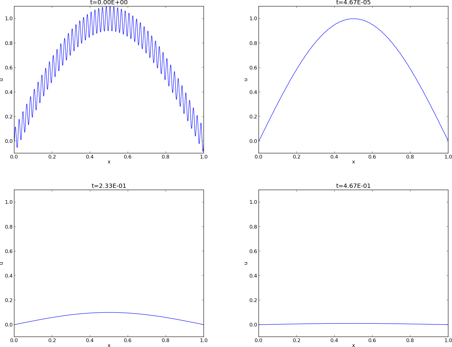
Evolution of the solution of a diffusion problem: initial condition (upper left), 1/100 reduction of the small waves (upper right), 1/10 reduction of the long wave (lower left), and 1/100 reduction of the long wave (lower right)

The relevance of studying the behavior of a particular solution of the form (10) is related to a Fourier representation of the solution. We first express the initial condition as a Fourier series

\[I(x) \approx \sum_{k\in K} b_k e^{ikx},\]

where $i=\sqrt{-1}$ and $K$ is a set of $k$ values needed to build $I(x)$ with sufficient accuracy from basic sinusoidal components $e^{ikx}$. Instead of using a specific sine or cosine function for the spatial variation, we use a complex exponential function to ease the hand calculations later. Letting $K$ contain infinitely many $k$ values makes the sum converge to $I(x)$ under reasonable assumptions on the smoothness of $I(x)$.

The corresponding solution $u$ can now be expressed as

(12)\[ u(x,t) \approx \sum_{k\in K} b_k e^{-\alpha k^2t}e^{ikx},\]\[ \thinspace .\]

Note that (11) is a special case of (12) where $K=\{\pi, 100\pi\}$, $b_{\pi}=1$, and $b_{100\pi}=0.1$.

Analysis of the finite difference schemes¶

We have seen that a general solution of the diffusion equation can be built as a linear combination of basic components

\[e^{-\alpha k^2t}e^{ikx} \thinspace .\]

A fundamental question is whether such components are also solutions of the finite difference schemes. This is indeed the case, but the amplitude $\exp{(-\alpha k^2t)}$ might be modified (which also happens when solving the ODE counterpart $u'=-\alpha u$). We therefore look for numerical solutions of the form

(13)\[ u^n_q = A^n e^{ikq\Delta x} = A^ne^{ikx},\]

where $A$ must be determined by inserting the component into an actual scheme.

Stability (1)¶

The exact wave component decays according to $\exp{(-\alpha k^2t)}$. We should therefore require $|A| < 1$ to have a decaying numerical solution as well. However, if $-1\leq A<0$, $A^n$ will change sign from time level to time level, and we get stable, non-physical oscillations in the numerical solutions that are not present in the exact solution.

Accuracy (1)¶

To determine how accurately a finite difference scheme treats one wave component (13), we see that the basic deviation from the exact solution is reflected in how well $A^n$ approximates $\exp{(-\alpha k^2t)}=\exp{(-\alpha k^2 n\Delta t)}$, or how well the numerical amplification factor $A$ approximates the exact amplification factor $A_{\small\mbox{e}} = \exp{(-\alpha k^2 \Delta t)}$.

Analysis of the Forward Euler scheme¶

The Forward Euler finite difference scheme for $u_t = \alpha u_{xx}$ can be written as

\[[D_t^+ u = \alpha D_xD_x u]^n_q\thinspace .\]

Inserting a wave component (13) in the scheme demands calculating the terms

\[e^{ikq\Delta x}[D_t^+ A]^n = e^{ikq\Delta x}A^n\frac{A-1}{\Delta t},\]

and

\[A^nD_xD_x [e^{ikx}]_q = A^n\left( - e^{ikq\Delta x}\frac{4}{\Delta x^2} \sin^2\left(\frac{k\Delta x}{2}\right)\right) \thinspace .\]

Inserting these terms in the discrete equation and dividing by $A^n e^{ikq\Delta x}$ leads to

\[\frac{A-1}{\Delta t} = -\alpha \frac{4}{\Delta x^2}\sin^2\left( \frac{k\Delta x}{2}\right),\]

and consequently

\[A = 1 -4C\sin^2\left( \frac{k\Delta x}{2}\right),\]

where $C$ is a constant introduced for convenience:

\[C = \frac{\alpha\Delta t}{\Delta x^2} \thinspace .\]

The complete numerical solution is then

\[u^n_q = \left(1 -4C\sin^2\left( \frac{k\Delta x}{2}\right)\right)^ne^{ikq\Delta x} \thinspace .\]

Stability (2)¶

We easily see that $A\leq 1$. However, the $A$ can be less than $-1$, which will lead to growth of a numerical wave component. The criterion $A\geq -1$ implies

\[4C\sin^2 (p/2)\leq 2 \thinspace .\]

The worst case is when $\sin^2 (p/2)=1$, so a sufficient criterion for stability is

\[C\leq \frac{1}{2},\]

or expressed as a condition on $\Delta t$:

\[\Delta t\leq \frac{\Delta x^2}{2\alpha}\thinspace .\]

Note that halving the spatial mesh size, $\Delta x \rightarrow \frac{1}{2} \Delta x$, requires $\Delta t$ to be reduced by a factor of $1/4$. The method hence becomes very expensive for fine spatial meshes.

Accuracy (2)¶

Since $A$ is expressed in terms of $C$ and the parameter we now call $p=k\Delta x$, we also express $A_{\small\mbox{e}}$ by $C$ and $p$:

\[A_{\small\mbox{e}} = \exp{(-\alpha k^2\Delta t)} = \exp{(-Cp^2)} \thinspace .\]

Computing the Taylor series expansion of $A/A_{\small\mbox{e}}$ in terms of $C$ can easily be done with aid of sympy:

def A_exact(C, p):
    return exp(-C*p**2)

def A_FE(C, p):
    return 1 - 4*C*sin(p/2)**2

from sympy import *
C, p = symbols('C p')
A_err_FE = A_FE(C, p)/A_exact(C, p)
print A_err_FE.series(C, 0, 6)

The result is

\[\frac{A}{A_{\small\mbox{e}}} = 1 - 4 C \sin^{2}(p/2) + C p^{2} - 4 C^{2} p^{2} \sin^{2}(p/2) + \frac{1}{2} C^{2} p^{4} + \cdots\]

Recalling that $C=\alpha\Delta t/\Delta x$, $p=k\Delta x$, and that $\sin^2(p/2)\leq 1$, we realize that the dominating error terms are at most

\[1 - 4\alpha \frac{\Delta t}{\Delta x^2} + \alpha\Delta t - 4\alpha^2\Delta t^2 + \alpha^2 \Delta t^2\Delta x^2 + \cdots \thinspace .\]

Analysis of the Backward Euler scheme¶

Discretizing $u_t = \alpha u_{xx}$ by a Backward Euler scheme,

\[[D_t^- u = \alpha D_xD_x u]^n_q,\]

and inserting a wave component (13), leads to calculations similar to those arising from the Forward Euler scheme, but since

\[e^{ikq\Delta x}[D_t^- A]^n = A^ne^{ikq\Delta x}\frac{1 - A^{-1}}{\Delta t},\]

we get

\[\frac{1-A^{-1}}{\Delta t} = -\alpha \frac{4}{\Delta x^2}\sin^2\left( \frac{k\Delta x}{2}\right),\]

and then

(14)\[ A = \left(1 + 4C\sin^2(p/2)\right)^{-1}\]\[ \thinspace .\]

The complete numerical solution can be written

\[u^n_q = \left(1 + 4C\sin^2 (p/2)\right)^{-n} e^{ikq\Delta x} \thinspace .\]

Stability (3)¶

We see from (14) that $0<A<1$, which means that all numerical wave components are stable and non-oscillatory for any $\Delta t >0$.

Analysis of the Crank-Nicolson scheme¶

The Crank-Nicolson scheme can be written as

\[[D_t u = \alpha D_xD_x \overline{u}^x]^{n+\frac{1}{2}}_q,\]

or

\[[D_t u]^{n+\frac{1}{2}}_q = \frac{1}{2}\alpha\left( [D_xD_x u]^{n}_q + [D_xD_x u]^{n+1}_q\right) \thinspace .\]

Inserting (13) in the time derivative approximation leads to

\[[D_t A^n e^{ikq\Delta x}]^{n+\frac{1}{2}} = A^{n+\frac{1}{2}} e^{ikq\Delta x}\frac{A^{\frac{1}{2}}-A^{-\frac{1}{2}}}{\Delta t} = A^ne^{ikq\Delta x}\frac{A-1}{\Delta t} \thinspace .\]

Inserting (13) in the other terms and dividing by $A^ne^{ikq\Delta x}$ gives the relation

\[\frac{A-1}{\Delta t} = -\frac{1}{2}\alpha\frac{4}{\Delta x^2} \sin^2\left(\frac{k\Delta x}{2}\right) (1 + A),\]

and after some more algebra,

\[A = \frac{ 1 - 2C\sin^2(p/2)}{1 + 2C\sin^2(p/2)} \thinspace .\]

The exact numerical solution is hence

\[u^n_q = \left(\frac{ 1 - 2C\sin^2(p/2)}{1 + 2C\sin^2(p/2)}\right)^ne^{ikp\Delta x} \thinspace .\]

Stability (4)¶

The criteria $A>-1$ and $A<1$ are fulfilled for any $\Delta t >0$.

Summary of accuracy of amplification factors¶

We can plot the various amplification factors against $p=k\Delta x$ for different choices of the $C$ parameter. Figures Amplification factors for large time steps, Amplification factors for time steps around the Forward Euler stability limit, and Amplification factors for small time steps show how long and small waves are damped by the various schemes compared to the exact damping. As long as all schemes are stable, the amplification factor is positive, except for Crank-Nicolson when $C>0.5$.

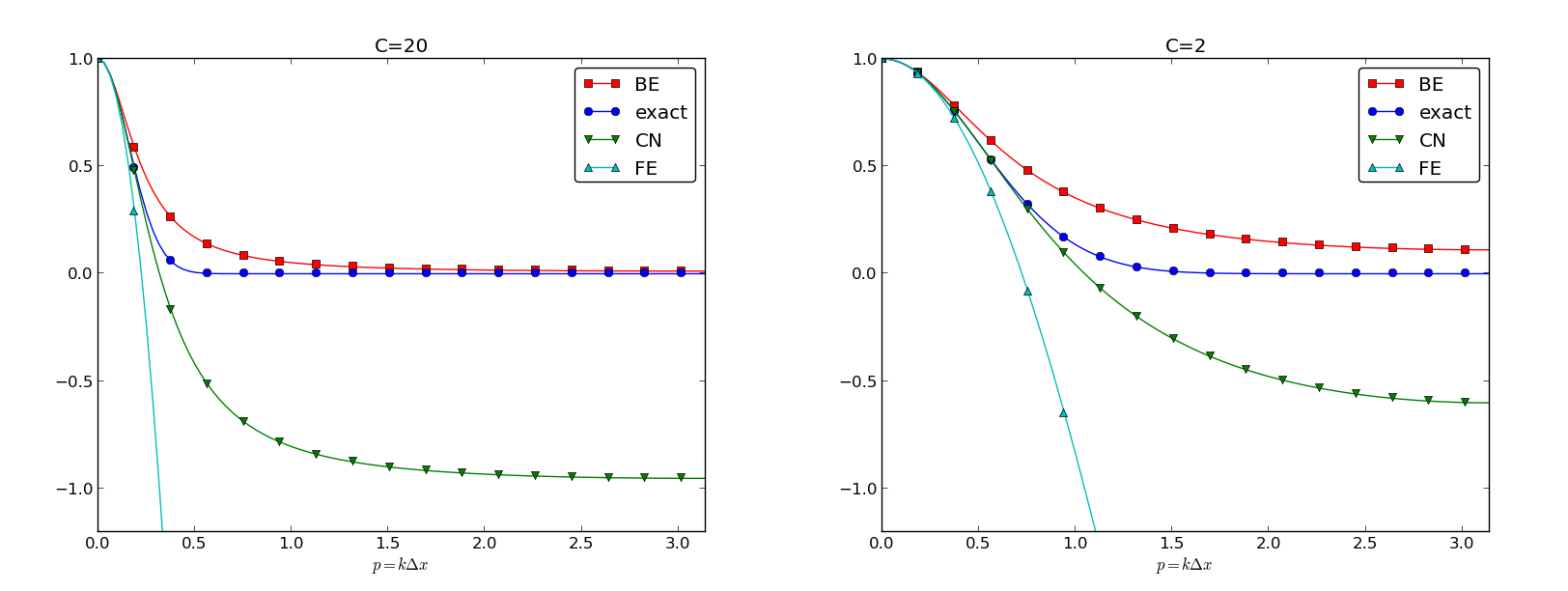
Amplification factors for large time steps

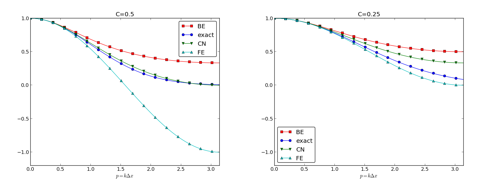
Amplification factors for time steps around the Forward Euler stability limit

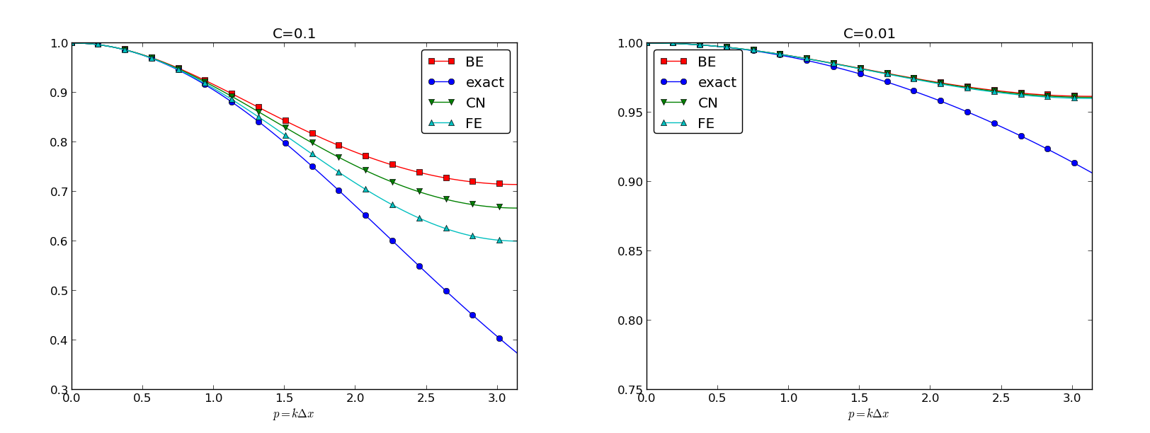
Amplification factors for small time steps

The effect of negative amplification factors is that $A^n$ changes sign from one time level to the next, thereby giving rise to oscillations in time in an animation of the solution. We see from Figure Amplification factors for large time steps that for $C=20$, waves with $p\geq \pi/2$ undergo a damping close to $-1$, which means that the amplitude does not decay and that the wave component jumps up and down in time. For $C=2$ we have a damping of a factor of 0.5 from one time level to the next, which is very much smaller than the exact damping. Short waves will therefore fail to be effectively dampened. These waves will manifest themselves as high frequency oscillatory noise in the solution.

A value $p=\pi/2$ corresponds to four mesh points per wave length of $e^{ikx}$, while $p=\pi$ implies only two points per wave length, which is the smallest number of points we can have to represent the wave on the mesh.

To demonstrate the oscillatory behavior of the Crank-Nicolson scheme, we choose an initial condition that leads to short waves with significant amplitude. A discontinuous $I(x)$ will in particular serve this purpose.

Run $C=...$...

Finite difference methods for diffusion processes¶

A simple 1D diffusion equation¶

Forward Euler scheme¶

Backward Euler Scheme¶

Sparse matrix implementation¶

The \(\theta\) Rule¶

The Laplace and Poisson equation as the steady state limit¶

Extensions¶

Analysis of schemes for the diffusion equation¶

Properties of the solution¶

Analysis of the finite difference schemes¶

Stability (1)¶

Accuracy (1)¶

Analysis of the Forward Euler scheme¶

Stability (2)¶

Accuracy (2)¶

Analysis of the Backward Euler scheme¶

Stability (3)¶

Analysis of the Crank-Nicolson scheme¶

Stability (4)¶

Summary of accuracy of amplification factors¶

Table Of Contents

Previous topic

Navigation

Finite difference methods for diffusion processes¶

A simple 1D diffusion equation¶

Forward Euler scheme¶

Backward Euler Scheme¶

Sparse matrix implementation¶

The \(\theta\) Rule¶

The Laplace and Poisson equation as the steady state limit¶

Extensions¶

Analysis of schemes for the diffusion equation¶

Properties of the solution¶

Analysis of the finite difference schemes¶

Stability (1)¶

Accuracy (1)¶

Analysis of the Forward Euler scheme¶

Stability (2)¶

Accuracy (2)¶

Analysis of the Backward Euler scheme¶

Stability (3)¶

Analysis of the Crank-Nicolson scheme¶

Stability (4)¶

Summary of accuracy of amplification factors¶

Table Of Contents

Previous topic

Quick search

Navigation