Finite difference methods for first-order ODEs
| Author: | Hans Petter Langtangen |
|---|---|
| Date: | Dec 13, 2012 |
Note: PRELIMINARY VERSION (expect typos!)
Finite difference methods for partial differential equations (PDEs) employ a range of concepts and tools that can be introduced and illustrated in the context of simple ordinary differential equation (ODE) examples. By first working with ODEs, we keep the mathematical problems to be solved as simple as possible (but no simpler), thereby allowing full focus on understanding the concepts and tools that will be reused and further extended when addressing finite difference methods for time-dependent PDEs. The forthcoming treatment of ODEs is therefore solely dominated by reasoning and methods that directly carry over to numerical methods for PDEs.
We study two model problems: an ODE for a decaying phenomena, which will be relevant for PDEs of diffusive nature, and an ODE for oscillating phenomena, which will be relevant for PDEs of wave nature. Both problems are linear with known analytical solutions such that we can easily assess the quality of various numerical methods and analyze their behavior.
Finite difference methods
The purpose of this module is to explain finite difference methods in detail for a simple ordinary differential equation (ODE). Emphasis is put on the reasoning when discretizing the problem, various ways of programming the methods, how to verify that the implementation is correct, experimental investigations of the numerical behavior of the methods, and theoretical analysis of the methods to explain the observations.
A basic model for exponential decay
Our model problem is perhaps the simplest ODE:
Here, \(a>0\) is a constant and \(u'(t)\) means differentiation with respect to time \(t\). This type of equation arises in a number of widely different phenomena where some quantity \(u\) undergoes exponential reduction. Examples include radioactive decay, population decay, investment decay, cooling of an object, pressure decay in the atmosphere, and retarded motion in fluids (for some of these models, \(a\) can be negative as well). Studying numerical solution methods for this simple ODE gives important insight that can be reused for diffusion PDEs.
The analytical solution of the ODE is found by the method of separation of variables, resulting in
for any arbitrary constant \(C\). To formulate a mathematical problem for which there is a unique solution, we need a condition to fix the value of \(C\). This condition is known as the initial condition and stated as \(u(0)=I\). That is, we know the value \(I\) of \(u\) when the process starts at \(t=0\). The exact solution is then \(u(t)=I\exp{(-at)}\).
We seek the solution \(u(t)\) of the ODE for \(t\in (0,T]\). The point \(t=0\) is not included since we know \(u\) here and assume that the equation governs \(u\) for \(t>0\). The complete ODE problem then reads: find \(u(t)\) such that
This is known as a continuous problem because the parameter \(t\) varies continuously from \(0\) to \(T\). For each \(t\) we have a corresponding \(u(t)\). There are hence infinitely many values of \(t\) and \(u(t)\). The purpose of a numerical method is to formulate a corresponding discrete problem whose solution is characterized by a finite number of values, which can be computed in a finite number of steps on a computer.
The Forward Euler scheme
Solving an ODE like (1) by a finite difference method consists of the following four steps:
- discretizing the domain,
- fulfilling the equation at discrete time points,
- replacing derivatives by finite differences,
- formulating a recursive algorithm.
Step 1: Discretizing the domain
The time domain \([0,T]\) is represented by a finite number of \(N+1\) points
The collection of points \(t_0,t_1,\ldots,t_N\) constitutes a mesh or grid. Often the mesh points will be uniformly spaced in the domain \([0,T]\), which means that the spacing \(t_{n+1}-t_n\) is the same for all \(n\). This spacing is then often denoted by \(\Delta t\), in this case \(t_n=n\Delta t\).
We seek the solution \(u\) at the mesh points: \(u(t_n)\), \(n=1,2,\ldots,N\) (note that \(u^0\) is already known as \(I\)). A notational short-form for \(u(t_n)\), which will be used extensively, is \(u^{n}\). More precisely, we let \(u^n\) be the numerical approximation to the exact solution at \(t=t_n\), \(u(t_n)\). When we need to clearly distinguish the numerical and the exact solution, we often place a subscript e on the exact solution, as in \({u_{\small\mbox{e}}}(t_n)\). Figure Time mesh with discrete solution values shows the \(t_n\) and \(u_n\) points for \(n=0,1,\ldots,N=7\) as well as \(u_{\small\mbox{e}}(t)\) as the dashed line.
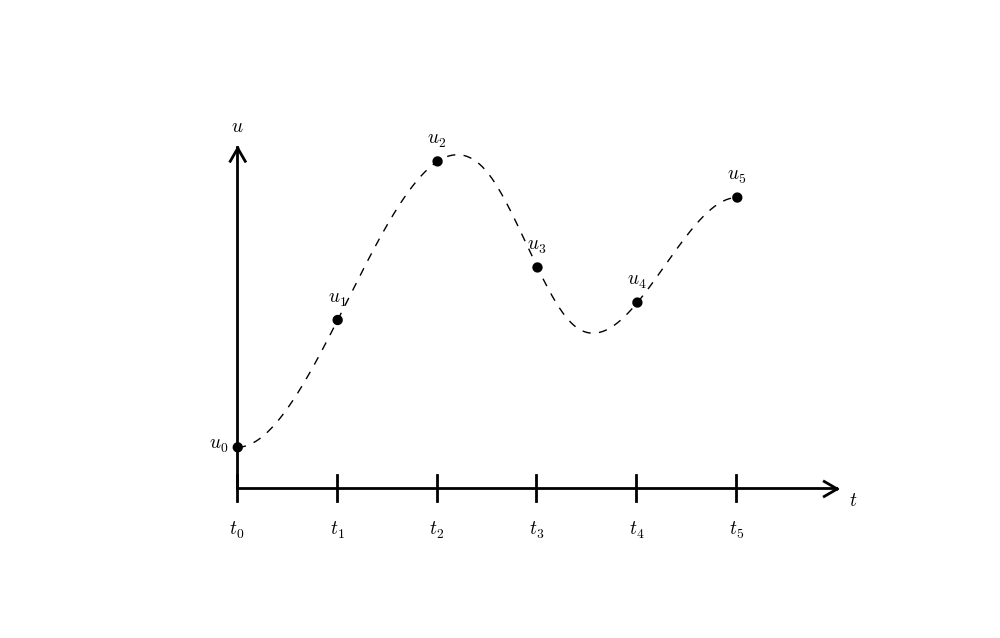
Time mesh with discrete solution values
Since finite difference methods produce solutions at the mesh points only, it is an open question what the solution is between the mesh points. One can use methods for interpolation to compute the value of \(u\) between mesh points. The simplest (and most widely used) interpolation method is to assume that \(u\) varies linearly between the mesh points, see Figure Linear interpolation between the discrete solution values (dashed curve is exact solution). Given \(u^{n}\) and \(u^{n+1}\), the value of \(u\) at some \(t\in [t_{n}, t_{n+1}]\) is by linear interpolation
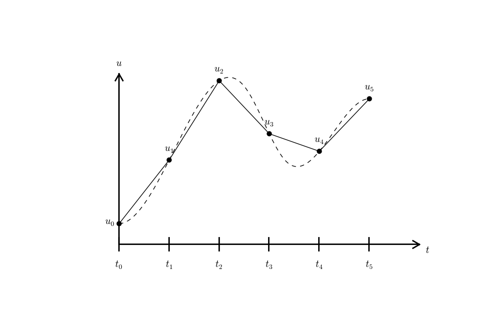
Linear interpolation between the discrete solution values (dashed curve is exact solution)
Step 2: Fulfilling the equation at discrete time points
The ODE is supposed to hold for all \(t\in (0,T]\), i.e., at an infinite number of points. Now we relax that requirement and require that the ODE is fulfilled at a finite set of discrete points in time. The mesh points \(t_1,t_2,\ldots,t_N\) are a natural choice of points. The original ODE is then reduced to the following \(N\) equations:
Step 3: Replacing derivatives by finite differences
The next and most essential step of the method is to replace the derivative \(u'\) by a finite difference approximation. Let us first try a one-sided difference approximation (see Figure Illustration of a forward difference),
Inserting this approximation in (2) results in
This equation is the discrete counterpart to the original ODE problem (1), and often known as a finite difference scheme, which yields a straightforward way to compute the solution at the mesh points (\(u(t_n)\), \(n=1,2,\ldots,N\)) as shown next.
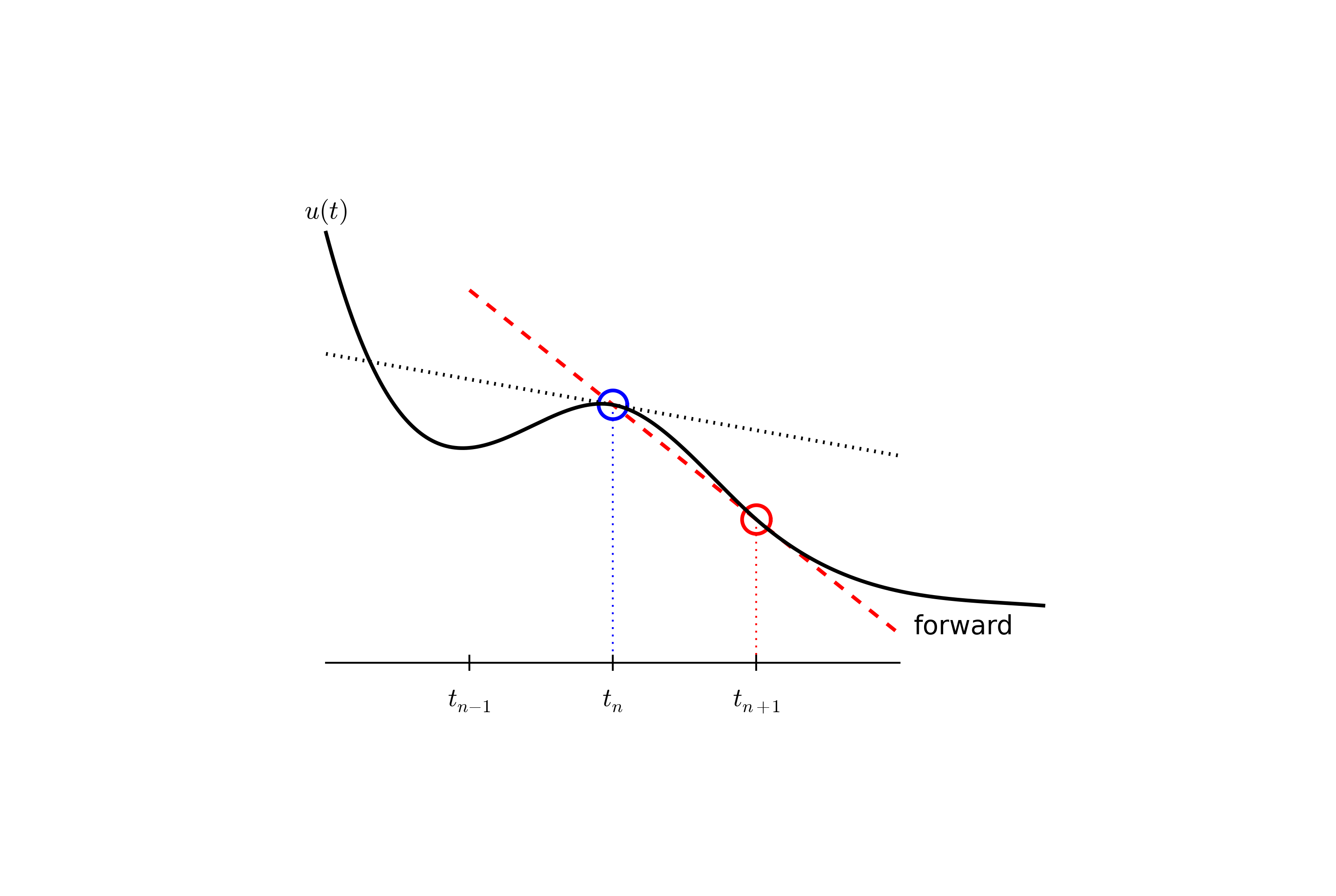
Illustration of a forward difference
Step 4: Formulating a recursive algorithm
The final step is to identify the computational algorithm to be implemented in a program. The key observation here is to realize that (4) can be used to compute \(u^{n+1}\) if \(u^n\) is known. Starting with \(n=0\), \(u^0\) is known since \(u^0=u(0)=I\), and (4) gives an equation for \(u^1\). Knowing \(u^1\), \(u^2\) can be found from (4). In general, \(u^n\) in (4) can be assumed known, and then we can easily solve for the unknown \(u^{n+1}\):
We shall refer to (5) as the Forward Euler (FE) scheme for our model problem. From a mathematical point of view, equations of the form (5) are known as difference equations since they express how differences in \(u\), like \(u^{n+1}-u^n\), evolve with \(n\). The finite difference method can be viewed as a method for turning a differential equation into a difference equation.
Computation with (5) is straightforward:
and so on until we reach \(u^N\). In the case \(t_{n+1}-t_n\) is a constant, denoted by \(\Delta t\), we realize from the above calculations that
This means that we have found a closed formula for \(u^n\), and there is no need to let a computer generate the sequence \(u^1, u^2, u^3, \ldots\). However, finding such a formula for \(u^n\) is possible only for a few very simple problems.
As the next sections will show, the scheme (5) is just one out of many alternative finite difference (and other) schemes for the model problem (1).
The Backward Euler scheme
There are many choices of difference approximations in step 3 of the finite difference method as presented in the previous section. Another alternative is
Since this difference is based on going backward in time (\(t_{n-1}\)) for information, it is known as the Backward Euler difference. Figure decay:sketch:BE explains the idea.
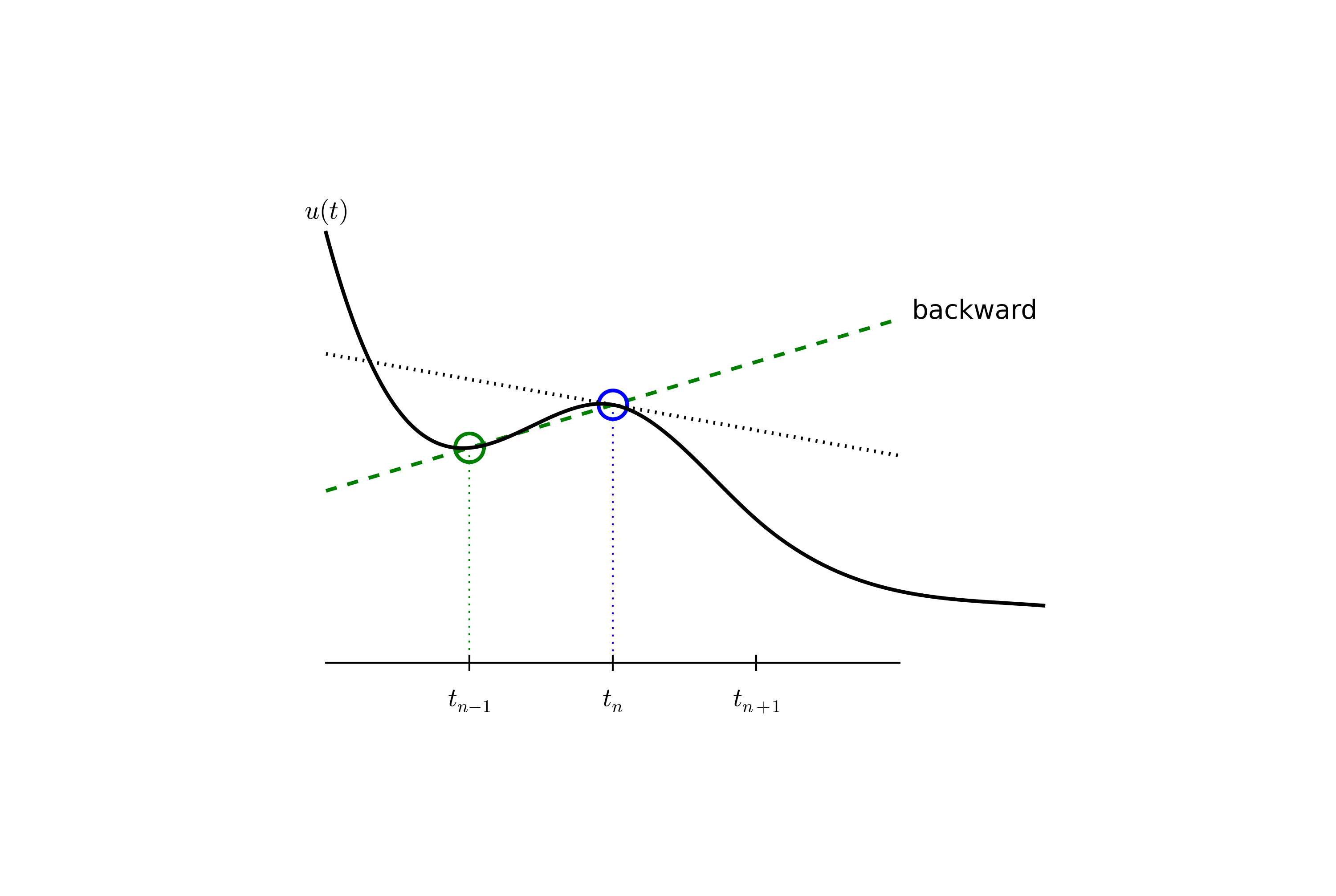
Illustration of a backward difference
Inserting (6) in (2) yields the Backward Euler (BE) scheme:
We assume, as explained under step 4 in the section The Forward Euler scheme, that we have computed \(u^0, u^1, \ldots, u^{n-1}\) such that (7) can be used to compute \(u^n\). For direct similarity with the Forward Euler scheme (5) we replace \(n\) by \(n+1\) in (7) and solve for the unknown value \(u^{n+1}\):
The Crank-Nicolson scheme
The finite difference approximations used to derive the schemes (5) and (8) are both one-sided differences, known to be less accurate than central (or midpoint) differences. We shall now construct a central difference at \(t_{n+1/2}=\frac{1}{2} (t_n + t_{n+1})\), or \(t_{n+1/2}=(n+\frac{1}{2})\Delta t\) if the mesh spacing is uniform in time. The approximation reads
Note that the fraction on the right-hand side is the same as for the Forward Euler approximation (3) and the Backward Euler approximation (6) (with \(n\) replaced by \(n+1\)). The accuracy of this fraction as an approximation to the derivative of \(u\) depends on where we seek the derivative: in the center of the interval \([t_{n},t_{n+1}]\) or at the end points.
With the formula (9), where \(u'\) is evaluated at \(t_{n+1/2}\), it is natural to demand the ODE to be fulfilled at the time points between the mesh points:
where \(u^{n+\frac{1}{2}}\) is a short form for \(u(t_{n+\frac{1}{2}})\). The problem is that we aim to compute \(u^n\) for integer \(n\), implying that \(u^{n+\frac{1}{2}}\) is not a quantity computed by our method. It must be expressed by the quantities that we actually produce, i.e., \(u\) at the mesh points. One possibility is to approximate \(u^{n+\frac{1}{2}}\) as an average of the \(u\) values at the neighboring mesh points:
Figure decay:sketch:BE sketches the geometric interpretation of such a centered difference.
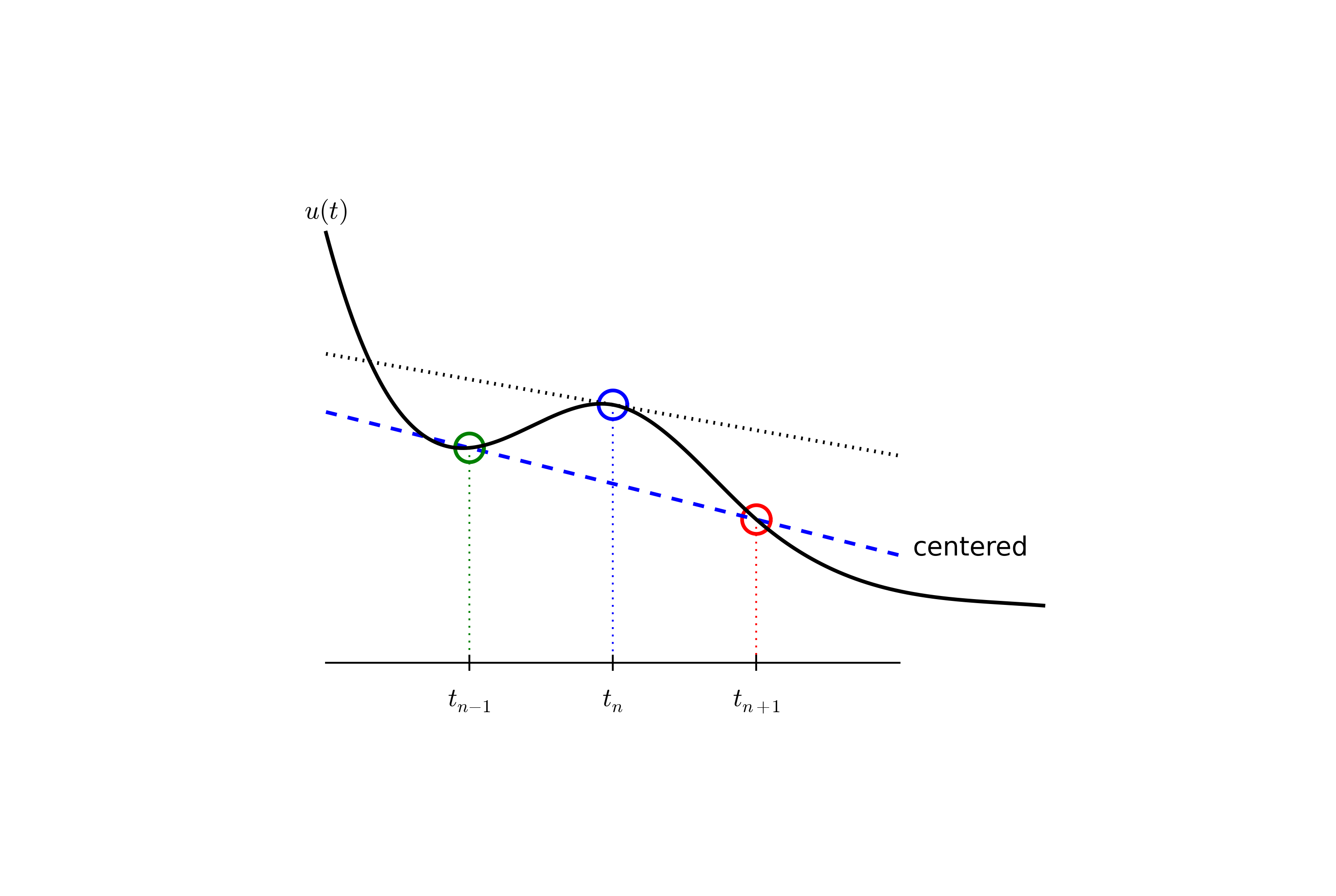
Illustration of a centered difference
We assume that \(u^n\) is already computed so that \(u^{n+1}\) is the unknown, which we can solve for:
The finite difference scheme (14) is known as the midpoint scheme or the Crank-Nicolson (CN) scheme. We shall use the latter name.
The unifying \(\theta\)-rule
Let us reconsider the derivation of the Forward Euler, Backward Euler, and Crank-Nicolson schemes. In all the mentioned schemes we replace \(u'\) by the fraction
and the difference between the methods lies in which point this fraction approximates the derivative; i.e., in which point we sample the ODE. So far this has been the end points or the midpoint of \([t_n,t_{n+1}]\). However, we may choose any point \(\tilde t \in [t_n,t_{n+1}]\). The difficulty is that evaluating the right-hand side \(-au\) at an arbitrary point faces the same problem as in the section The Crank-Nicolson scheme: the point value must be expressed by the discrete \(u\) quantities that we compute by the scheme, i.e., \(u^n\) and \(u^{n+1}\). Following the averaging idea from the section The Crank-Nicolson scheme, the value of \(u\) at an arbitrary point \(\tilde t\) can be calculated as a weighted average, which generalizes the arithmetic average \(\frac{1}{2}u^n + \frac{1}{2}u^{n+1}\). If we express \(\tilde t\) as a weighted average
where \(\theta\in [0,1]\) is the weighting factor, we can write
We can now let the ODE hold at the point \(\tilde t\in [t_n,t_{n+1}]\), approximate \(u'\) by the fraction \((u^{n+1}-u^{n})/(t_{n+1}-t_n)\), and approximate the right-hand side \(-au\) by the weighted average (15). The result is
This is a generalized scheme for our model problem: \(\theta =0\) gives the Forward Euler scheme, \(\theta =1\) gives the Backward Euler scheme, and \(\theta =1/2\) gives the Crank-Nicolson scheme. In addition, we may choose any other value of \(\theta\) in \([0,1]\).
As before, \(u^n\) is considered known and \(u^{n+1}\) unknown, so we solve for the latter:
This scheme is known as the \(\theta\)-rule, or alternatively written as the “theta-rule”.
Constant time step
All schemes up to now have been formulated for a general non-uniform mesh in time: \(t_0,t_1,\ldots,t_N\). Non-uniform meshes are highly relevant since one can use many points in regions where \(u\) varies rapidly, and save points in regions where \(u\) is slowly varying. This is the key idea of adaptive methods where the spacing of the mesh points are determined as the computations proceed.
However, a uniformly distributed set of mesh points is very common and sufficient for many applications. It therefore makes sense to present the finite difference schemes for a uniform point distribution \(t_n=n\Delta t\), where \(\Delta t\) is the constant spacing between the mesh points, also referred to as the time step. The resulting formulas look simpler and are perhaps more well known:
Not surprisingly, we present alternative schemes because they have different pros and cons, both for the simple ODE in question (which can easily be solved as accurately as desired), and for more advanced differential equation problems.
Compact operator notation for finite differences
Finite difference formulas can be tedious to write and read, especially for differential equations with many terms and many derivatives. To save space and help the reader of the scheme to quickly see the nature of the difference approximations, we introduce a compact notation. A forward difference approximation is denoted by the \(D_t^+\) operator:
The notation consists of an operator that approximates differentiation with respect to an independent variable, here \(t\). The operator is built of the symbol \(D\), with the variable as subscript and a superscript denoting the type of difference. The superscript \({}^+\) indicates a forward difference. We place square brackets around the operator and the function it operates on and specify the mesh point, where the operator is acting, by a superscript.
The corresponding operator notation for a centered difference and a backward difference reads
and
Note that the superscript \({}^-\) denotes the backward difference, while no superscript implies a central difference.
An averaging operator is also convenient to have:
The superscript \(t\) indicates that the average is taken along the time coordinate. The common average \((u^n + u^{n+1})/2\) can now be expressed as \([\overline{u}^{t}]^{n+1/2}\).
The Backward Euler finite difference approximation to \(u'=-au\) can be written as follows utilizing the compact notation:
In difference equations we often place the square brackets around the whole equation, to indicate at which mesh point the equation applies, since each term is supposed to be approximated at the same point:
The Forward Euler scheme takes the form
while the Crank-Nicolson scheme is written as
Just apply (19) and (21) and write out the expressions to see that (22) is indeed the Crank-Nicolson scheme.
The \(\theta\)-rule can be specified by
if we define a new time difference and a weighted averaging operator:
where \(\theta\in [0,1]\). Note that for \(\theta =1/2\) we recover the standard centered difference and the standard arithmetic average. The idea in (23) is to sample the equation at \(t_{n+\theta}\), use a skew difference at that point \([\bar D_t u]^{n+\theta}\), and a shifted mean value. An alternative notation is
Looking at the various examples above and comparing them with the underlying differential equations, we see immediately which difference approximations that have been used and at which point they apply. Therefore, the compact notation efficiently communicates the reasoning behind turning a differential equation into a difference equation.
Implementation (1)
The purpose now is to make a computer program for solving
and display the solution on the screen, preferably together with the exact solution. We shall also be concerned with how we can test that the implementation is correct.
All programs referred to in this section are found in the src/decay directory.
Mathematical problem. We want to explore the Forward Euler scheme, the Backward Euler, and the Crank-Nicolson schemes applied to our model problem. From an implementational points of view, it is advantageous to implement the \(\theta\)-rule
since it can generate the three other schemes by various of choices of \(\theta\): \(\theta=0\) for Forward Euler, \(\theta =1\) for Backward Euler, and \(\theta =1/2\) for Crank-Nicolson. Given \(a\), \(u^0=I\), \(T\), and \(\Delta t\), our task is to use the \(\theta\)-rule to compute \(u^1, u^2,\ldots,u^N\), where \(t_N=N\Delta t\), and \(N\) the closest integer to \(T/\Delta t\).
Computer Language: Python. Any programming language can be used to generate the \(u^{n+1}\) values from the formula above. However, in this document we shall mainly make use of Python of several reasons:
- Python has a very clean, readable syntax (often known as “executable pseudo-code”).
- Python code is very similar to MATLAB code (and MATLAB has a particularly widespread use for scientific computing).
- Python is similar to, but much simpler to work with and results in more reliable code than C++.
- Python is a full-fledged, very powerful programming language.
- Python has a rich set of modules for scientific computing, and its popularity in scientific computing is rapidly growing.
- Python was made for being combined with compiled languages (C, C++, Fortran) to reuse existing numerical software and to reach high computational performance of new implementations.
- Python has extensive support for administrative task needed when doing large-scale computational investigations.
- Python has extensive support for graphics (visualization, user interfaces, web applications).
- FEniCS, a very powerful tool for solving PDEs by the finite element method, is most human-efficient to operate from Python.
Learning Python is easy. Many newcomers to the language will probably learn enough from the examples to perform their own computer experiments. The examples start with simple Python code and gradually make use of more powerful constructs as we proceed. As long as it is not inconvenient for the problem at hand, our Python code is made as close as possible to MATLAB code for easy transition between the two languages.
Making a solver function
We choose to have an array u for storing the \(u^n\) values, \(n=0,1,\ldots,N\). The algorithmic steps are
- initialize \(u^0\)
- for \(t=t_n\), \(n=1,2,\ldots,N\): compute \(u_n\) using the \(\theta\)-rule formula
Function for computing the numerical solution
The following Python function takes the input data of the problem (\(I\), \(a\), \(T\), \(\Delta t\), \(\theta\)) as arguments and returns two arrays with the solution \(u^0,\ldots,u^N\) and the mesh points \(t_0,\ldots,t_N\), respectively:
from numpy import *

def solver(I, a, T, dt, theta):
    """Solve u'=-a*u, u(0)=I, for t in (0,T] with steps of dt."""
    N = int(T/dt)            # no of time intervals
    T = N*dt                 # adjust T to fit time step dt
    u = zeros(N+1)           # array of u[n] values
    t = linspace(0, T, N+1)  # time mesh

    u[0] = I                 # assign initial condition
    for n in range(0, N):    # n=0,1,...,N-1
        u[n+1] = (1 - (1-theta)*a*dt)/(1 + theta*dt*a)*u[n]
    return u, t
The numpy library contains a lot of functions for array computing. Most of the function names are similar to what is found in the alternative scientific computing language MATLAB. Here we make use of
- zeros(N+1) for creating an array of a size N+1 and initializing the elements to zero
- linspace(0, T, N+1) for creating an array with N+1 coordinates uniformly distributed between 0 and T
The for loop deserves a comment, especially for newcomers to Python. The construction range(0, N, s) generates all integers from 0 to N in steps of s, but not including N. Omitting s means s=1. For example, range(0, 6, 3) gives 0 and 3, while range(0, N) generates 0, 1, ..., N-1. In our loop, n takes on the values generated by range(0, N), implying the following assignments u[n+1]: u[1], u[2], ..., u[N], which is what we want since u has length N+1. The first index in Python arrays or lists is always 0 and the last is then len(u)-1.
To compute with the solver function, we need to call it. Here is a sample call:
u, t = solver(I=1, a=2, T=8, dt=0.8, theta=1)
Integer division
The shown implementation of the solver may face problems and wrong results if T, a, dt, and theta are given as integers, see Exercise 1: Experiment with integer division and Exercise 2: Experiment with wrong computations. The problem is related to integer division in Python (as well as in Fortran, C, and C++): 1/2 becomes 0, while 1.0/2, 1/2.0, or 1.0/2.0 all become are 0.5. It is enough that at least the nominator or the denominator is a real number (i.e., a float object) to ensure correct mathematical division. Inserting a conversion dt = float(dt) guarantees that dt is float and avoids problems in Exercise 2: Experiment with wrong computations.
Another problem with computing \(N=T/\Delta t\) is that we should round \(N\) to the nearest integer. With N = int(T/dt) the int operation picks the largest integer smaller than T/dt. Correct rounding is obtained by
N = int(round(T/dt))
The complete version of our improved, safer solver function then becomes
from numpy import *

def solver(I, a, T, dt, theta):
    """Solve u'=-a*u, u(0)=I, for t in (0,T] with steps of dt."""
    dt = float(dt)           # avoid integer division
    N = int(round(T/dt))     # no of time intervals
    T = N*dt                 # adjust T to fit time step dt
    u = zeros(N+1)           # array of u[n] values
    t = linspace(0, T, N+1)  # time mesh

    u[0] = I                 # assign initial condition
    for n in range(0, N):    # n=0,1,...,N-1
        u[n+1] = (1 - (1-theta)*a*dt)/(1 + theta*dt*a)*u[n]
    return u, t
Doc strings
Right below the header line in the solver function there is a Python string enclosed in triple double quotes """. The purpose of this string object is to document what the function does and what the arguments are. In this case the necessary documentation do not span more than one line, but with triple double quoted strings the text may span several lines:
def solver(I, a, T, dt, theta):
    """
    Solve

        u'(t) = -a*u(t),

    with initial condition u(0)=I, for t in the time interval
    (0,T]. The time interval is divided into time steps of
    length dt.

    theta=1 corresponds to the Backward Euler scheme, theta=0
    to the Forward Euler scheme, and theta=0.5 to the Crank-
    Nicolson method.
    """
    ...
Such documentation strings appearing right after the header of a function are called doc strings. There are tools that can automatically produce nicely formatted documentation by extracting the definition of functions and the contents of doc strings.
It is strongly recommended to equip any function whose purpose is not obvious with a doc string. Nevertheless, the forthcoming text deviates from this rule if the function is explained in the text.
Formatting of numbers
Having computed the discrete solution u, it is natural to look at the numbers:
# Write out a table of t and u values:
for i in range(len(t)):
    print t[i], u[i]
This compact print statement gives unfortunately quite ugly output because the t and u values are not aligned in nicely formatted columns. To fix this problem, we recommend to use the printf format, supported most programming languages inherited from C. Another choice is Python’s recent format string syntax.
Writing t[i] and u[i] in two nicely formatted columns is done like this with the printf format:
print 't=%6.3f u=%g' % (t[i], u[i])
The percentage signs signify “slots” in the text where the variables listed at the end of the statement are inserted. For each “slot” one must specify a format for how the variable is going to appear in the string: s for pure text, d for an integer, g for a real number written as compactly as possible, 9.3E for scientific notation with three decimals in a field of width 9 characters (e.g., -1.351E-2), or .2f for a standard decimal notation, here with two decimals, formatted with minimum width. The printf syntax provides a quick way of formatting tabular output of numbers with full control of the layout.
The alternative format string syntax looks like
print 't={t:6.3f} u={u:g}'.format(t=t[i], u=u[i])
As seen, this format allows logical names in the “slots” where t[i] and u[i] are to be inserted. The “slots” are surrounded by curly braces, and the logical name is followed by a colon and then the printf-like specification of how to format real numbers, integers, or strings.
Running the program
The function and main program shown above must be placed in a file, say with name dc_v1.py. Make sure you write the code with a suitable text editor (Gedit, Emacs, Vim, Notepad++, or similar). The program is run by executing the file this way:
Terminal> python dc_v1.py
The text Terminal> just signifies a prompt in a Unix/Linux or DOS terminal window. After this prompt (which will look different in your terminal window, depending on the terminal application and how it is set up), commands like python dc_v1.py can be issued. These commands are interpreted by the operating system.
We strongly recommend to run Python programs within the IPython shell. First start IPython by typing ipython in the terminal window. Inside the IPython shell, our program dc_v1.py is run by the command run dc_v1.py. The advantage of running programs in IPython are many: previous commands are easily recalled, %pdb turns on debugging so that variables can be examined if the program aborts due to an exception, output of commands are stored in variables, programs and statements can be profiled, any operating system command can be executed, modules can be loaded automatically and other customizations can be performed when starting IPython – to mention a few of the most useful features.
Although running programs in IPython is strongly recommended, most execution examples in the forthcoming text use the standard Python shell with prompt >>> and run programs through a typesetting like Terminal> python programname. The reason is that such typesetting makes the text more compact in the vertical direction than showing sessions with IPython syntax.
Verifying the implementation
It is easy to make mistakes while deriving and implementing numerical algorithms, so we should never believe in the printed \(u\) values before they have been thoroughly verified. The most obvious idea is to compare the computed solution with the exact solution, when that exists, but there will always be a discrepancy between these two solutions because of the numerical approximations. The challenging question is whether we have the mathematically correct discrepancy or if we have another, maybe small, discrepancy due to both an approximation error and an error in the implementation.
The purpose of verifying a program is to bring evidence for the fact that there are no errors in the implementation. To avoid mixing unavoidable approximation errors and undesired implementation errors, we should try to make tests where we have some exact computation of the discrete solution or at least parts of it.
Running a few algorithmic steps by hand
The simplest approach to produce a correct reference for the discrete solution \(u\) of finite difference equations is to compute a few steps of the algorithm by hand. Then we can compare the hand calculations with numbers produced by the program.
A straightforward approach is to use a calculator and compute \(u^1\), \(u^2\), and \(u^3\). However, the chosen values of \(I\) and \(\theta\) given in the execution example above are not good, because the numbers 0 and 1 can easily simplify formulas too much for test purposes. For example, with \(\theta =1\) the nominator in the formula for \(u^n\) will be the same for all \(a\) and \(\Delta t\) values. One should therefore choose more “arbitrary” values, say \(\theta =0.8\) and \(I=0.1\). Hand calculations with the aid of a calculator gives
Comparison of these manual calculations with the result of the solver function is carried out in the function
def verify_three_steps():
    """Compare three steps with known manual computations."""
    theta = 0.8; a = 2; I = 0.1; dt = 0.8
    u_by_hand = array([I,
                       0.0298245614035,
                       0.00889504462912,
                       0.00265290804728])

    N = 3  # number of time steps
    u, t = solver(I=I, a=a, T=N*dt, dt=dt, theta=theta)

    tol = 1E-15  # tolerance for comparing floats
    difference = abs(u - u_by_hand).max()
    success = difference <= tol
    return success
The main program, where we call the solver function and print u, is now put in a separate function main:
def main():
    u, t = solver(I=1, a=2, T=8, dt=0.8, theta=1)
    # Write out a table of t and u values:
    for i in range(len(t)):
        print 't=%6.3f u=%g' % (t[i], u[i])
        # or print 't={t:6.3f} u={u:g}'.format(t=t[i], u=u[i])
The main program in the file may now first run the verification test and then go on with the real simulation (main()) only if the test is passed:
if verify_three_steps():
    main()
else:
    print 'Bug in the implementation!'
Since the verification test is always done, future errors introduced accidentally in the program have a good chance of being detected.
It is essential that verification tests can be automatically run at any time. For this purpose, there are test frameworks and corresponding programming rules that allow us to request running through a suite of test cases, but in this very early stage of program development we just implement and run the verification in our own code so that every detail is visible and understood.
The complete program including the verify_three_steps* functions is found in the file dc_verf1.py.
Comparison with an exact discrete solution
Sometimes it is possible to find a closed-form exact discrete solution that fulfills the discrete finite difference equations. The implementation can then be verified against the exact discrete solution. This is usually the best technique for verification.
Define
Manual computations with the \(\theta\)-rule results in
We have then established the exact discrete solution as
One should be conscious about the different meanings of the notation on the left- and right-hand side of this equation: on the left, \(n\) is a superscript reflecting a counter of mesh points, while on the right, \(n\) is the power in an exponentiation.
Comparison of the exact discrete solution and the computed solution is done in the following function:
def verify_exact_discrete_solution():

    def exact_discrete_solution(n, I, a, theta, dt):
        factor = (1 - (1-theta)*a*dt)/(1 + theta*dt*a)
        return I*factor**n

    theta = 0.8; a = 2; I = 0.1; dt = 0.8
    N = int(8/dt)  # no of steps
    u, t = solver(I=I, a=a, T=N*dt, dt=dt, theta=theta)
    u_de = array([exact_discrete_solution(n, I, a, theta, dt)
                  for n in range(N+1)])
    difference = abs(u_de - u).max()  # max deviation
    tol = 1E-15  # tolerance for comparing floats
    success = difference <= tol
    return success
Note that one can define a function inside another function (but such a function is invisible outside the function in which it is defined). The complete program is found in the file dc_verf2.py.
Computing the numerical error
Now that we have evidence for a correct implementation, we are in a position to compare the computed \(u^n\) values in the u array with the exact \(u\) values at the mesh points, in order to study the error in the numerical solution.
Let us first make a function for the analytical solution \(u_{\small\mbox{e}}(t)=Ie^{-at}\) of the model problem:
def exact_solution(t, I, a):
    return I*exp(-a*t)
A natural way to compare the exact and discrete solutions is to calculate their difference at the mesh points:
These numbers are conveniently computed by
u, t = solver(I, a, T, dt, theta)  # Numerical solution
u_e = exact_solution(t, I, a)
e = u_e - u
The last two statements make use of array arithmetics: t is an array of mesh points that we pass to exact_solution. This function evaluates -a*t, which is a scalar times an array, meaning that the scalar is multiplied with each array element. The result is an array, let us call it tmp1. Then exp(tmp1) means applying the exponential function to each element in tmp, resulting an array, say tmp2. Finally, I*tmp2 is computed (scalar times array) and u_e refers to this array returned from exact_solution. The expression u_e - u is the difference between two arrays, resulting in a new array referred to by e.
The array e is the current problem’s discrete error function. Very often we want to work with just one number reflecting the size of the error. A common choice is to integrate \(e_n^2\) over the mesh and take the square root. Assuming the exact and discrete solution to vary linearly between the mesh points, the integral is given exactly by the Trapezoidal rule:
A common approximation of this expression, for convenience, is
The error in this approximation is not much of a concern: it means that the error measure is not exactly the Trapezoidal rule of an integral, but a slightly different measure. We could equally well have chosen other error messages, but the choice is not important as long as we use the same error measure consistently in all experiments when investigating the error.
The error measure \(\hat E\) or \(E\) is referred to as the \(L_2\) norm of the discrete error function. The formula for \(E\) will be frequently used:
The corresponding Python code, using array arithmetics, reads
E = sqrt(dt*sum(e**2))
The sum function comes from numpy and computes the sum of the elements of an array. Also the sqrt function is from numpy and computes the square root of each element in the array argument.
Instead of doing array computing we can compute with one element at a time:
m = len(u)     # length of u array (alt: u.size)
u_e = zeros(m)
t = 0
for i in range(m):
    u_e[i] = exact_solution(t, a, I)
    t = t + dt
e = zeros(m)
for i in range(m):
    e[i] = u_e[i] - u[i]
s = 0  # summation variable
for i in range(m):
    s = s + e[i]**2
error = sqrt(dt*s)
Such element-wise computing, often called scalar computing, takes more code, is less readable, and runs much slower than array computing.
Plotting solutions
Having the t and u arrays, the approximate solution u is visualized by plot(t, u):
from matplotlib.pyplot import *
plot(t, u)
show()
It will be illustrative to also plot \(u_{\small\mbox{e}}(t)\) for comparison. Doing a plot(t, u_e) is not exactly what we want: the plot function draws straight lines between the discrete points (t[n], u_e[n]) while \(u_{\small\mbox{e}}(t)\) varies as an exponential function between the mesh points. The technique for showing the “exact” variation of \(u_{\small\mbox{e}}(t)\) between the mesh points is to introduce a very fine mesh for \(u_{\small\mbox{e}}(t)\):
t_e = linspace(0, T, 1001)      # fine mesh
u_e = exact_solution(t_e, I, a)
plot(t,   u,   'r-')            # red  line for u
plot(t_e, u_e, 'b-')            # blue line for u_e
With more than one curve in the plot we need to associate each curve with a legend. We also want appropriate names on the axis, a title, and a file containing the plot as an image for inclusion in reports. The Matplotlib package (matplotlib.pyplot) contains functions for this purpose. The names of the functions are similar to the plotting functions known from MATLAB. A complete plot session then becomes
from matplotlib.pyplot import *

figure()                          # create new plot
t_e = linspace(0, T, 1001)        # fine mesh for u_e
u_e = exact_solution(t_e, I, a)
plot(t,   u,   'r--o')            # red dashes w/circles
plot(t_e, u_e, 'b-')              # blue line for exact sol.
legend(['numerical', 'exact'])
xlabel('t')
ylabel('u')
title('theta=%g, dt=%g' % (theta, dt))
savefig('%s_%g.png' % (theta, dt))
show()
Note that savefig here creates a PNG file whose name reflects the values of \(\theta\) and \(\Delta t\) so that we can easily distinguish files from different runs with \(\theta\) and \(\Delta t\).
A bit more sophisticated and easy-to-read filename can be generated by mapping the \(\theta\) value to acronyms for the three common schemes: FE (Forward Euler, \(\theta=0\)), BE (Backward Euler, \(\theta=1\)), CN (Crank-Nicolson, \(\theta=0.5\)). A Python dictionary is ideal for such a mapping from numbers to strings:
theta2name = {0: 'FE', 1: 'BE', 0.5: 'CN'}
savefig('%s_%g.png' % (theta2name[theta], dt))
Let us wrap up the computation of the error measure and all the plotting statements in a function explore. This function can be called for various \(\theta\) and \(\Delta t\) values to see how the error varies with the method and the mesh resolution:
def explore(I, a, T, dt, theta=0.5, makeplot=True):
    """
    Run a case with the solver, compute error measure,
    and plot the numerical and exact solutions (if makeplot=True).
    """
    u, t = solver(I, a, T, dt, theta)  # Numerical solution
    u_e = exact_solution(t, I, a)
    e = u_e - u
    E = sqrt(dt*sum(e**2))
    if makeplot:
        figure()                         # create new plot
        t_e = linspace(0, T, 1001)       # fine mesh for u_e
        u_e = exact_solution(t_e, I, a)
        plot(t,   u,   'r--o')           # red dashes w/circles
        plot(t_e, u_e, 'b-')             # blue line for exact sol.
        legend(['numerical', 'exact'])
        xlabel('t')
        ylabel('u')
        title('theta=%g, dt=%g' % (theta, dt))
        theta2name = {0: 'FE', 1: 'BE', 0.5: 'CN'}
        savefig('%s_%g.png' % (theta2name[theta], dt))
        savefig('%s_%g.pdf' % (theta2name[theta], dt))
        savefig('%s_%g.eps' % (theta2name[theta], dt))
        show()
    return E
The figure() call is key here: without it, a new plot command will draw the new pair of curves in the same plot window, while we want the different pairs to appear in separate windows and files. Calling figure() ensures this.
The explore function stores the plot in three different image file formats: PNG, PDF, and EPS (Encapsulated PostScript). The PNG format is aimed at being included in HTML files, the PDF format in pdfLaTeX documents, and the EPS format in LaTeX documents. Frequently used viewers for these image files on Unix systems are gv (comes with Ghostscript) for the PDF and EPS formats and display (from the ImageMagick) suite for PNG files:
Terminal> gv BE_0.5.pdf
Terminal> gv BE_0.5.eps
Terminal> display BE_0.5.png
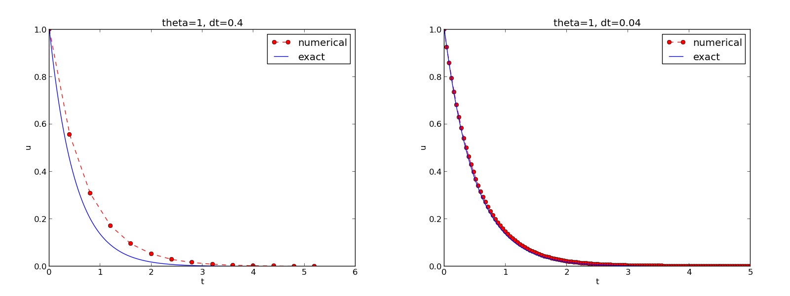
The complete code containing the functions above resides in the file dc_plot_mpl.py. Running this program results in
Terminal> python dc_plot_mpl.py
0.0   0.40:    2.105E-01
0.0   0.04:    1.449E-02
0.5   0.40:    3.362E-02
0.5   0.04:    1.887E-04
1.0   0.40:    1.030E-01
1.0   0.04:    1.382E-02
We observe that reducing \(\Delta t\) by a factor of 10 increases the accuracy for all three methods (\(\theta\) values). We also see that the combination of \(\theta=0.5\) and a small time step \(\Delta t =0.04\) gives a much more accurate solution, and that \(\theta=0\) and \(\theta=0\) with \(\Delta t = 0.4\) result in the least accurate solutions.
Figure The Forward Euler scheme for two values of the time step demonstrates that the numerical solution for \(\Delta t=0.4\) clearly lies below the exact curve, but that the accuracy improves considerably by using 1/10 of this time step.
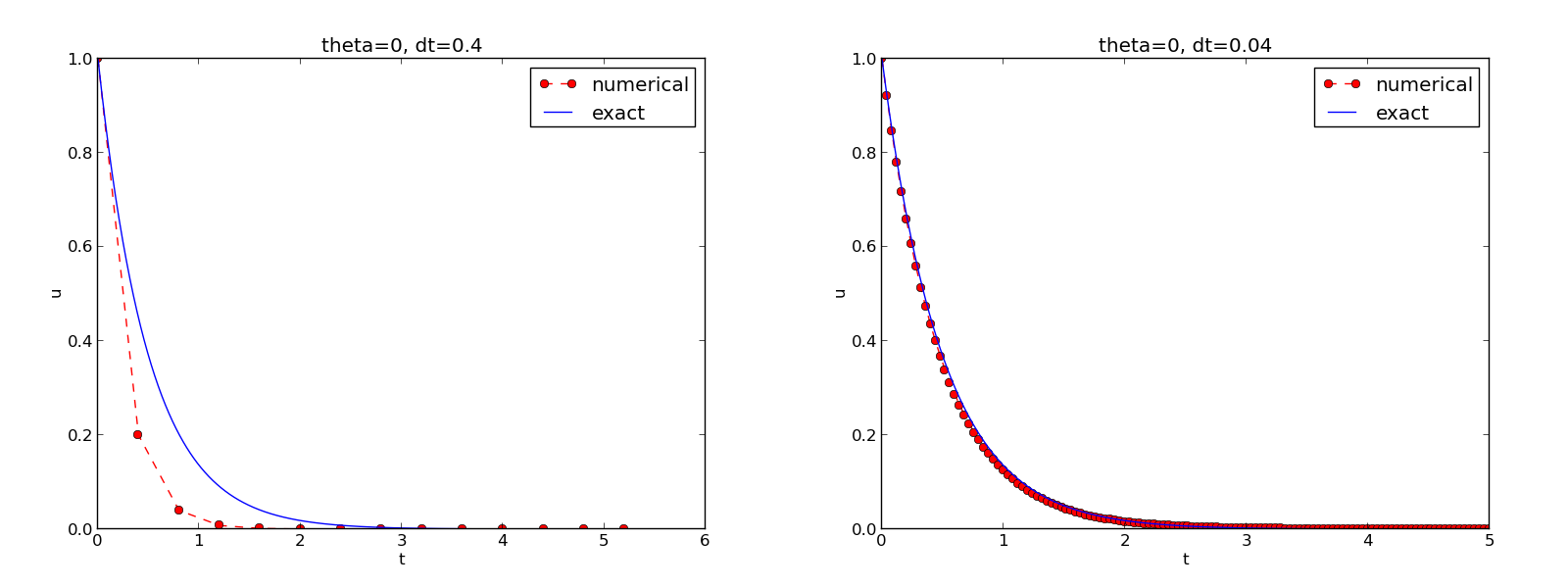
The Forward Euler scheme for two values of the time step
Mounting two PNG files, as done in the figure, is easily done by the montage program from the ImageMagick suite:
Terminal> montage -background white -geometry 100% -tile 2x1 \
          FE_0.4.png FE_0.04.png FE1.png
Terminal> convert -trim FE1.png FE1.png
The -geometry argument is used to specify the size of the image, and here we preserve the individual sizes of the images. The -tile HxV option specifies H images in the horizontal direction and V images in the vertical direction. A series of image files to be combined are then listed, with the name of the resulting combined image, here FE1.png at the end. The convert -trim command removes surrounding white areas in the figure.
For LaTeX{} reports it is not recommended to use montage and PNG files as the result has too low resolution. Instead, plots should be made in the PDF format and combined using the pdftk, pdfnup, and pdfcrop tools (on Linux/Unix):
Terminal> pdftk FE_0.4.png FE_0.04.png output tmp.pdf
Terminal> pdfnup --nup 2x1 tmp.pdf     # output in tmp-nup.pdf
Terminal> pdfcrop tmp-nup.pdf tmp.pdf  # output in tmp.pdf
Terminal> mv tmp.pdf FE1.png
Here, pdftk combines images into a multi-page PDF file, pdfnup combines the images in individual pages to a table of images (pages), and pdfcrop removes white margins in the resulting combined image file.
The behavior of the two other schemes is shown in Figures The Backward Euler scheme for two values of the time step and The Crank-Nicolson scheme for two values of the time step. Crank-Nicolson is obviously the most accurate scheme from this visual point of view.
The Backward Euler scheme for two values of the time step

The Crank-Nicolson scheme for two values of the time step
Plotting with SciTools
The SciTools package provides a unified plotting interface, called Easyviz, to many different plotting packages, including Matplotlib. The syntax is very similar to that of Matplotlib and MATLAB. In fact, the plotting commands shown above look the same in SciTool’s Easyviz interface, apart from the import statement, which reads
from scitools.std import *
This statement performs a from numpy import * as well as an import of the most common pieces of the Easyviz (scitools.easyviz) package, along with some additional numerical functionality.
With Easyviz one can, using an extended plot command, merge several plotting commands into one, using keyword arguments:
plot(t,   u,   'r--o',           # red dashes w/circles
     t_e, u_e, 'b-',             # blue line for exact sol.
     legend=['numerical', 'exact'],
     xlabel='t',
     ylabel='u',
     title='theta=%g, dt=%g' % (theta, dt),
     savefig='%s_%g.png' % (theta2name[theta], dt),
     show=True)
The dc_plot_st.py file contains such a demo.
By default, Easyviz employs Matplotlib for plotting, but Gnuplot and Grace are viable alternatives:
Terminal> python dc_plot_st.py --SCITOOLS_easyviz_backend gnuplot
Terminal> python dc_plot_st.py --SCITOOLS_easyviz_backend grace
The backend used for creating plots (and numerous other options) can be permanently set in SciTool’s configuration file.
All the Gnuplot windows are launched without any need to kill one before the next one pops up (as is the case with Matplotlib) and one can press the key ‘q’ anywhere in a plot window to kill it. Another advantage of Gnuplot is the automatic choice of sensible and distinguishable line types in black-and-white PostScript files (produced by savefig('myplot.eps')).
Regarding functionality for annotating plots with title, labels on the axis, legends, etc., we refer to the documentation of Matplotlib and SciTools for more detailed information on the syntax. The hope is that the programming syntax explained so far suffices for understanding the code and learning more from a combination of the forthcoming examples and other resources such as books and web pages.
Creating user interfaces
It is good programming practice to let programs read input from the user rather than require the user to edit the source code when trying out new values of input parameters. Reading input from the command line is a simple and flexible way of interacting with the user. Python stores all the command-line arguments in the list sys.argv, and there are, in principle, two ways of programming with command-line arguments in Python:
- Decide upon a sequence of parameters on the command line and read their values directly from the sys.argv[1:] list (sys.argv[0] is the just program name).
- Use option-value pairs (--option value) on the command line to override default values of input parameters, and use the argparse.ArgumentParser tool to interact with the command line.
Both strategies will be illustrated next.
Reading a sequence of command-line arguments
The dc_plot_mpl.py program needs the following input data: \(I\), \(a\), \(T\), an option to turn the plot on or off (makeplot), and a list of \(\Delta t\) values.
The simplest way of reading this input from the command line is to say that the first four command-line arguments correspond to the first four points in the list above, in that order, and that the rest of the command-line arguments are the \(\Delta t\) values. The input given for makeplot can be a string among 'on', 'off', 'True', and 'False'. The code for reading this input is most conveniently put in a function:
import sys

def read_command_line():
    if len(sys.argv) < 6:
        print 'Usage: %s I a T on/off dt1 dt2 dt3 ...' % \
              sys.argv[0]; sys.exit(1)  # abort

    I = float(sys.argv[1])
    a = float(sys.argv[2])
    T = float(sys.argv[3])
    makeplot = sys.argv[4] in ('on', 'True')
    dt_values = [float(arg) for arg in sys.argv[5:]]

    return I, a, T, makeplot, dt_values
One should note the following about the constructions in the program above:
- Everything on the command line ends up in a string in the list sys.argv. Explicit conversion to, e.g., a float object is required if the string as a number we want to compute with.
- The value of makeplot is determined from a boolean expression, which becomes True if the command-line argument is either 'on' or 'True', and False otherwise.
- It is easy to build the list of \(\Delta t\) values: we simply run through the rest of the list, sys.argv[5:], convert each command-line argument to float, and collect these float objects in a list, using the compact and convenient list comprehension syntax in Python.
The loops over \(\theta\) and \(\Delta t\) values can be coded in a main function:
def main():
    I, a, T, makeplot, dt_values = read_command_line()
    for theta in 0, 0.5, 1:
        for dt in dt_values:
            E = explore(I, a, T, dt, theta, makeplot)
            print '%3.1f %6.2f: %12.3E' % (theta, dt, E)
The complete program can be found in dc_cml.py.
Working with an argument parser
Python’s ArgumentParser tool in the argparse module makes it easy to create a professional command-line interface to any program. The documentation of `ArgumentParser <http://docs.python.org/library/argparse.html>`_ demonstrates its versatile applications, so we shall here just list an example containing the most used features. On the command line we want to specify option value pairs for \(I\), \(a\), and \(T\), e.g., --a 3.5 --I 2 --T 2. Including --makeplot turns the plot on and excluding this option turns the plot off. The \(\Delta t\) values can be given as --dt 1 0.5 0.25 0.1 0.01. Each parameter must have a sensible default value so that we specify the option on the command line only when the default value is not suitable.
We introduce a function for defining the mentioned command-line options:
def define_command_line_options():
    import argparse
    parser = argparse.ArgumentParser()
    parser.add_argument('--I', '--initial_condition', type=float,
                        default=1.0, help='initial condition, u(0)',
                        metavar='I')
    parser.add_argument('--a', type=float,
                        default=1.0, help='coefficient in ODE',
                        metavar='a')
    parser.add_argument('--T', '--stop_time', type=float,
                        default=1.0, help='end time of simulation',
                        metavar='T')
    parser.add_argument('--makeplot', action='store_true',
                        help='display plot or not')
    parser.add_argument('--dt', '--time_step_values', type=float,
                        default=[1.0], help='time step values',
                        metavar='dt', nargs='+', dest='dt_values')
    return parser
Each command-line option is defined through the parser.add_argument method. Alternative options, like the short --I and the more explaining version --initial_condition can be defined. Other arguments are type for the Python object type, a default value, and a help string, which gets printed if the command-line argument -h or --help is included. The metavar argument specifies the value associated with the option when the help string is printed. For example, the option for \(I\) has this help output:
Terminal> python dc_argparse.py -h
  ...
  --I I, --initial_condition I
                        initial condition, u(0)
  ...
The structure of this output is
--I metavar, --initial_condition metavar
                      help-string
The --makeplot option is a pure flag without any value, implying a true value if the flag is present and otherwise a false value. The action='store_true' makes an option for such a flag.
Finally, the --dt option demonstrates how to allow for more than one value (separated by blanks) through the nargs='+' keyword argument. After the command line is parsed, we get an object where the values of the options are stored as attributes. The attribute name is specified by the dist keyword argument, which for the --dt option reads dt_values. Without the dest argument, the value of option --opt is stored as the attribute opt.
The code below demonstrates how to read the command line and extract the values for each option:
def read_command_line():
    parser = define_command_line_options()
    args = parser.parse_args()
    print 'I={}, a={}, T={}, makeplot={}, dt_values={}'.format(
        args.I, args.a, args.T, args.makeplot, args.dt_values)
    return args.I, args.a, args.T, args.makeplot, args.dt_values
The main function remains the same as in the dc_cml.py code based on reading from sys.argv directly. A complete program using the demo above of ArgumentParser appears in the file dc_argparse.py.
Computing convergence rates
We normally expect that the error \(E\) in the numerical solution is reduced if the mesh size \(\Delta t\) is decreased. More specifically, many numerical methods obey a power-law relation between \(E\) and \(\Delta t\):
where \(C\) and \(r\) are (usually unknown) constants independent of \(\Delta t\). The formula (26) is viewed as an asymptotic model valid for sufficiently small \(\Delta t\). How small is normally hard to estimate without doing numerical estimations of \(r\).
The parameter \(r\) is known as the convergence rate. For example, if the convergence rate is 2, halving \(\Delta t\) reduces the error by a factor of 4. Diminishing \(\Delta t\) then has a greater impact on the error compared with methods that have \(r=1\). For a given value of \(r\), we refer to the method as of \(r\)-th order. First- and second-order methods are most common in scientific computing.
Estimating \(r\)
There are two ways of estimating \(C\) and \(r\) based on a set of \(m\) simulations with corresponding pairs \((\Delta t_i, E_i)\), \(i=0,\ldots,m-1\), and \(\Delta t_{i} < \Delta t_{i-1}\) (i.e., decreasing cell size).
- Take the logarithm of (26), \(\ln E = r\ln \Delta t + \ln C\), and fit a straight line to the data points \((\Delta t_i, E_i)\), \(i=0,\ldots,m-1\).
- Consider two consecutive experiments, \((\Delta t_i, E_i)\) and \((\Delta t_{i-1}, E_{i-1})\). Dividing the equation \(E_{i-1}=C\Delta t_{i-1}^r\) by \(E_{i}=C\Delta t_{i}^r\) and solving for \(r\) yields
for \(i=1,=\ldots,m-1\).
The disadvantage of method 1 is that (26) might not be valid for the coarsest meshes (largest \(\Delta t\) values), and fitting a line to all the data points is then misleading. Method 2 computes convergence rates for pairs of experiments and allows us to see if the sequence \(r_i\) converges to some value as \(i\rightarrow m-2\). The final \(r_{m-2}\) can then be taken as the convergence rate. If the coarsest meshes have a differing rate, the corresponding time steps are probably too large for (26) to be valid. That is, those time steps lie outside the asymptotic range of \(\Delta t\) values where the error behave like (26).
Implementation (2)
It is straightforward to extend the main function in the program dc_argparse.py with statements for computing \(r_0, r_1, \ldots, r_{m-2}\) from (26):
from math import log

def main():
    I, a, T, makeplot, dt_values = read_command_line()
    r = {}  # estimated convergence rates
    for theta in 0, 0.5, 1:
        E_values = []
        for dt in dt_values:
            E = explore(I, a, T, dt, theta, makeplot=False)
            E_values.append(E)

        # Compute convergence rates
        m = len(dt_values)
        r[theta] = [log(E_values[i-1]/E_values[i])/
                    log(dt_values[i-1]/dt_values[i])
                    for i in range(1, m, 1)]

    for theta in r:
        print '\nPairwise convergence rates for theta=%g:' % theta
        print ' '.join(['%.2f' % r_ for r_ in r[theta]])
    return r
The program is called dc_convrate.py.
The r object is a dictionary of lists. The keys in this dictionary are the \(\theta\) values. For example, r[1] holds the list of the \(r_i\) values corresponding to \(\theta=1\). In the loop for theta in r, the loop variable theta takes on the values of the keys in the dictionary r (in an undetermined ordering). We could simply do a print r[theta] inside the loop, but this would typically yield output of the convergence rates with 16 decimals:
[1.331919482274763, 1.1488178494691532, ...]
Instead, we format each number with 2 decimals, using a list comprehension to turn the list of numbers, r[theta], into a list of formatted strings. Then we join these strings with a space in between to get a sequence of rates on one line in the terminal window. More generally, d.join(list) joins the strings in the list list to one string, with d as delimiter between list[0], list[1], etc.
Here is an example on the outcome of the convergence rate computations:
Terminal> python dc_convrate.py --dt 0.5 0.25 0.1 0.05 0.025 0.01
...
Pairwise convergence rates for theta=0:
1.33 1.15 1.07 1.03 1.02

Pairwise convergence rates for theta=0.5:
2.14 2.07 2.03 2.01 2.01

Pairwise convergence rates for theta=1:
0.98 0.99 0.99 1.00 1.00
The Forward and Backward Euler methods seem to have an \(r\) value which stabilizes at 1, while the Crank-Nicolson seems to be a second-order method with \(r=2\).
Very often, we have some theory that predicts what \(r\) is for a numerical method. Various theoretical error measures for the \(\theta\)-rule point to \(r=2\) for \(\theta =0.5\) and \(r=1\) otherwise. The computed estimates of \(r\) are in very good agreement with these theoretical values.
The strong practical application of computing convergence rates is for verification: wrong convergence rates point to errors in the code, and correct convergence rates brings evidence that the implementation is correct. Experience shows that bugs in the code easily destroys the expected convergence rate.
Debugging via convergence rates
Let us experiment with bugs and see the implication on the convergence rate. We may, for instance, forget to multiply by a in the denominator in the updating formula for u[n+1]:
u[n+1] = (1 - (1-theta)*a*dt)/(1 + theta*dt)*u[n]
Running the same dc_convrate.py command as above gives the expected convergence rates (!). Why? The reason is that we just specified the \(\Delta t\) values are relied on default values for other parameters. The default value of \(a\) is 1. Forgetting the factor a has then no effect. This example shows how importance it is to avoid parameters that are 1 or 0 when verifying implementations. Running the code dc_v0.py with \(a=2.1\) and \(I=0.1\) yields
Terminal> python dc_convrate.py --a 2.1 --I 0.1  \
          --dt 0.5 0.25 0.1 0.05 0.025 0.01
...
Pairwise convergence rates for theta=0:
1.49 1.18 1.07 1.04 1.02

Pairwise convergence rates for theta=0.5:
-1.42 -0.22 -0.07 -0.03 -0.01

Pairwise convergence rates for theta=1:
0.21 0.12 0.06 0.03 0.01
This time we see that the expected convergence rates for the Crank-Nicolson and Backward Euler methods are not obtained, while \(r=1\) for the Forward Euler method. The reason for correct rate in the latter case is that \(\theta=0\) and the wrong theta*dt term in the denominator vanishes anyway.
The error
u[n+1] = ((1-theta)*a*dt)/(1 + theta*dt*a)*u[n]
manifests itself through wrong rates \(r\approx 0\) for all three methods. About the same results arise from an erroneous initial condition, u[0] = 1, or wrong loop limits, range(1,N). It seems that in this simple problem, most bugs we can think of are detected by the convergence rate test, provided the values of the input data do not hide the bug.
A verify_convergence_rate function could compute the dictionary of list via main and check if the final rate estimates (\(r_{m-2}\)) are sufficiently close to the expected ones. A tolerance of 0.1 seems appropriate, given the uncertainty in estimating \(r\):
def verify_convergence_rate():
    r = main()
    tol = 0.1
    expected_rates = {0: 1, 1: 1, 0.5: 2}
    for theta in r:
        r_final = r[theta][-1]
        diff = abs(expected_rates[theta] - r_final)
        if diff > tol:
            return False
    return True  # all tests passed
We remark that r[theta] is a list and the last element in any list can be extracted by the index -1.
Memory-saving implementation
The memory storage requirements of our implementations so far consists mainly of the u and t arrays, both of length \(N+1\), plus some other temporary arrays that Python needs for intermediate results if we do array arithmetics in our program (e.g., I*exp(-a*t) needs to store a*t before - can be applied to it and then exp). The extremely modest storage requirements of simple ODE problems put no restrictions on the formulations of the algorithm and implementation. Nevertheless, when the methods for ODEs used here are applied to three-dimensional partial differential equation (PDE) problems, memory storage requirements suddenly become an issue.
The PDE counterpart to our model problem \(u'=-a\) is a diffusion equation \(u_t = a\nabla^2 u\) posed on a space-time domain. The discrete representation of this domain may in 3D be a spatial mesh of \(M^3\) points and a time mesh of \(N\) points. A typical desired value for \(M\) is 100 in many applications, or even \(1000\). Storing all the computed \(u\) values, like we have done in the programs so far, demands storage of some arrays of size \(M^3N\), giving a factor of \(M^3\) larger storage demands compared to our ODE programs. Each real number in the array for \(u\) requires 8 bytes of storage, resulting in a demand for 8 Gb of memory for only one array. In such cases one needs good ideas on how to lower the storage requirements. Fortunately, we can usually get rid of the \(M^3\) factor. Below we explain how this is done, and the technique is almost always applied in implementations of PDE problems.
Let us critically evaluate how much we really need to store in the computer’s memory in our implementation of the \(\theta\) method. To compute a new \(u^{n+1}\), all we need is \(u^n\). This implies that the previous \(u^{n-1},u^{n-2},\dots,u^0\) values do not need to be stored in an array, although this is convenient for plotting and data analysis in the program. Instead of the u array we can work with two variables for real numbers, u and u_1, representing \(u^{n+1}\) and \(u^n\) in the algorithm, respectively. At each time level, we update u from u_1 and then set u_1 = u so that the computed \(u^{n+1}\) value becomes the “previous” value \(u^n\) at the next time level. The downside is that we cannot plot the solution after the simulation is done since only the last two numbers are available. The remedy is to store computed values in a file and use the file for visualizing the solution later.
We have implemented this memory saving idea in the file dc_memsave.py, which is a merge of the dc_plot_mpl.py and dc_argparse.py programs, using module prefixes np for numpy and plt for matplotlib.pyplot.
The following function implements the ideas above regarding minimizing memory usage and storing the solution on file:
def solver_memsave(I, a, T, dt, theta, filename='sol.dat'):
    """
    Solve u'=-a*u, u(0)=I, for t in (0,T] with steps of dt.
    Minimum use of memory. The solution is store on file
    (with name filename) for later plotting.
    """
    dt = float(dt)        # avoid integer division
    N = int(round(T/dt))  # no of intervals

    outfile = open(filename, 'w')
    # u: time level n+1, u_1: time level n
    t = 0
    u_1 = I
    outfile.write('%.16E  %.16E\n' % (t, u_1))
    for n in range(1, N+1):
        u = (1 - (1-theta)*a*dt)/(1 + theta*dt*a)*u_1
        u_1 = u
        t += dt
        outfile.write('%.16E  %.16E\n' % (t, u))
    outfile.close()
    return u, t
This code snippet serves as a quick introduction to file writing in Python. Reading the data in the file into arrays t and u are done by the function
def read_file(filename='sol.dat'):
    infile = open(filename, 'r')
    u = [];  t = []
    for line in infile:
        words = line.split()
        if len(words) != 2:
            print 'Found more than two numbers on a line!', words
            sys.exit(1)  # abort
        t.append(float(words[0]))
        u.append(float(words[1]))
    return np.array(t), np.array(u)
This type of file with numbers in rows and columns is very common, and numpy has a function loadtxt which loads such tabular data into a two-dimensional array, say data. The number in row i and column j is then data[i,j]. The whole column number j can be extracted by data[:,j]. A version of read_file using np.loadtxt reads
def read_file_numpy(filename='sol.dat'):
    data = np.loadtxt(filename)
    t = data[:,0]
    u = data[:,1]
    return t, u
The present counterpart to the explore function from dc_plot_mpl.py must run solver_memsave and then load data from file before we can compute the error measure and make the plot:
def explore(I, a, T, dt, theta=0.5, makeplot=True):
    filename = 'u.dat'
    u, t = solver_memsave(I, a, T, dt, theta, filename)

    t, u = read_file(filename)
    u_e = exact_solution(t, I, a)
    e = u_e - u
    E = np.sqrt(dt*np.sum(e**2))
    if makeplot:
        plt.figure()
        ...
The dc_memsave.py file also includes command-line options --I, --a, --T, --dt, --theta, and --makeplot for controlling input parameters and making a single run. For example,
Terminal> python dc_memsave.py --T 10 --theta 1 --dt 2
I=1.0, a=1.0, T=10.0, makeplot=True, theta=1.0, dt=2.0
theta=1.0 dt=2 Error=3.136E-01
Software engineering
Efficient use of differential equation models requires software that is easy to test and flexible for setting up extensive numerical experiments. This section introduces three important concepts and their applications to the exponential decay model:
- Modules
- Testing frameworks
- Implementation with classes
Making a module
The previous sections has outlined numerous different programs, all of them having their own copy of the solver function. Such copies of the same piece of code is against the important Don’t Repeat Yourself (DRY) principle in programming. If we want to change the solver function there should be one and only one place where the change needs to be performed.
To clean up the repetitive code snippets scattered among the dc_*.py files, we start by collecting the various functions we want to keep for the future in one file, now called dc_mod.py. The following functions are copied to this file:
- solver
- verify_three_steps
- verify_discrete_solution
- explore
- define_command_line_options
- read_command_line extended to work both with sys.argv directly and with an ArgumentParser object
- main (with convergence rates estimation as in dc_convrate.py)
- verify_convergence_rate
We use Matplotlib for plotting. A sketch of the dc_mod.py file, with complete versions of the modified functions, looks as follows:
from numpy import *
from matplotlib.pyplot import *
import sys

def solver(I, a, T, dt, theta):
    ...

def verify_three_steps():
    ...

def verify_exact_discrete_solution():
    ...

def exact_solution(t, I, a):
    ...

def explore(I, a, T, dt, theta=0.5, makeplot=True):
    ...

def define_command_line_options():
    ...

def read_command_line(use_argparse=True):
    if use_argparse:
        parser = define_command_line_options()
        args = parser.parse_args()
        print 'I={}, a={}, makeplot={}, dt_values={}'.format(
            args.I, args.a, args.makeplot, args.dt_values)
        return args.I, args.a, args.makeplot, args.dt_values
    else:
        if len(sys.argv) < 6:
            print 'Usage: %s I a on/off dt1 dt2 dt3 ...' % \
                  sys.argv[0]; sys.exit(1)

        I = float(sys.argv[1])
        a = float(sys.argv[2])
        T = float(sys.argv[3])
        makeplot = sys.argv[4] in ('on', 'True')
        dt_values = [float(arg) for arg in sys.argv[5:]]

        return I, a, makeplot, dt_values

def main():
    ...
This dc_mod.py file is already a module such that we can import desired in functions in other programs. For example,
from decay_theta import solver
u, t = solver(I=1.0, a=3.0, T=3, dt=0.01, theta=0.5)
However, it should also be possible to both use dc_mod.py as a module and execute the file as a program that runs main(). This is accomplished by ending the file with a test block:
if __name__ == '__main__':
    main()
When dc_mod.py is used as a module, __name__ equals the module name decay_theta, while __name__ equals '__main__' when the file is run as a program. Optionally, we could run the verification tests if the word verify is present on the command line and verify_convergence_rate could be tested if verify_rates is found on the command line. The verify_rates argument must be removed before we read parameter values from the command line, other wise read_command_line (called by main) will not work properly.
if __name__ == '__main__':
    if 'verify' in sys.argv:
        if verify_three_steps() and verify_discrete_solution():
            pass # ok
        else:
            print 'Bug in the implementation!'
    elif 'verify_rates' in sys.argv:
        sys.argv.remove('verify_rates')
        if not '--dt' in sys.argv:
            print 'Must assign several dt values'
            sys.exit(1)  # abort
        if verify_convergence_rate():
            pass
        else:
            print 'Bug in the implementation!'
    else:
        # Perform simulations
        main()
Prefixing imported functions by the module name
Import statements of the form from module import * imports functions and variables in module.py into the current file. For example, when doing
from numpy import *
from matplotlib.pyplot import *
we get mathematical functions like sin and exp as well as MATLAB-style functions like linspace and plot, which can be called by these well-known names. However, it sometimes becomes confusing to know where a particular function comes from. Is it from numpy? Or matplotlib.pyplot? Or is it our own function?
An alternative import is
import numpy
import matplotlib.pyplot
and such imports require functions to be prefixed by the module name, e.g.,
t = numpy.linspace(0, T, N+1)
u_e = I*numpy.exp(-a*t)
matplotlib.pyplot.plot(t, u_e)
This is normally regarded as a better habit because it is explicitly stated from which module a function comes from.
The modules numpy and matplotlib.pyplot are so frequently used, and their full names quite tedious to write, so two standard abbreviations have evolved in the Python scientific computing community:
import numpy as np
import matplotlib.pyplot as plt

t = np.linspace(0, T, N+1)
u_e = I*np.exp(-a*t)
plt.plot(t, u_e)
A version of the decay_theta module where we use the np and plt prefixes is found in the file decay_theta_v2.py.
The downside of prefixing functions by the module name is that mathematical expressions like \(e^{-at}\sin(2\pi t)\) gets cluttered with module names,
numpy.exp(-a*t)*numpy.sin(2(numpy.pi*t)
# or
np.exp(-a*t)*np.sin(2*np.pi*t)
Such an expression looks like exp(-a*t)*sin(2*pi*t) in most other programming languages. Similarly, np.linspace and plt.plot look less familiar to people who are used to MATLAB and who have not adopted Python’s prefix style. Whether to do from module import * or import module depends on personal taste and the problem at hand. In these writings we use from module import in shorter programs where similarity with MATLAB could be an advantage, and where a one-to-one correspondence between mathematical formulas and Python expressions is important. The style import module is preferred inside Python modules (see Exercise 9: Make a module for a demonstration).
Doctests
We have emphasized how important it is to be able to run tests in the program at any time. This was solved by calling various verify* functions in the previous examples. However, there exists well-established procedures and corresponding tools for automating checking of tests. We shall briefly demonstrate two important techniques: doctest and unit testing. The corresponding files are the modules dc_mod_doctest.py and dc_mod_unittest.py.
Doc strings (the first string after the function header) are used to document the purpose of functions and their arguments. Very often it is instructive to include an example on how to use the function. Interactive examples in the Python shell are most illustrative as we can see the output resulting from function calls. For example, we can in the solver function include an example on calling this function and printing the computed u and t arrays:
def solver(I, a, T, dt, theta):
    """
    Solve u'=-a*u, u(0)=I, for t in (0,T] with steps of dt.


    >>> u, t = solver(I=0.8, a=1.2, T=4, dt=0.5, theta=0.5)
    >>> for t_n, u_n in zip(t, u):
    ...     print 't=%.1f, u=%.14f' % (t_n, u_n)
    t=0.0, u=0.80000000000000
    t=0.5, u=0.43076923076923
    t=1.0, u=0.23195266272189
    t=1.5, u=0.12489758761948
    t=2.0, u=0.06725254717972
    t=2.5, u=0.03621291001985
    t=3.0, u=0.01949925924146
    t=3.5, u=0.01049960113002
    t=4.0, u=0.00565363137770
    """
    ...
When such interactive demonstrations are inserted in doc strings, Python’s doctest module can be used to automate running all commands in interactive sessions and compare new output with the output appearing in the doc string. All we have to do in the current example is to write
Terminal> python -m doctest dc_mod_doctest.py
This command imports the doctest module, which runs all tests. No additional command-line argument is allowed when running doctest. If any test fails, the problem is reported, e.g.,
Terminal> python -m doctest dc_mod_doctest.py
********************************************************
File "dc_mod_doctest.py", line 12, in dc_mod_doctest....
Failed example:
    for t_n, u_n in zip(t, u):
        print 't=%.1f, u=%.14f' % (t_n, u_n)
Expected:
    t=0.0, u=0.80000000000000
    t=0.5, u=0.43076923076923
    t=1.0, u=0.23195266272189
    t=1.5, u=0.12489758761948
    t=2.0, u=0.06725254717972
    t=2.5, u=0.03621291001985
    t=3.0, u=0.01949925924146
    t=3.5, u=0.01049960113002
    t=4.0, u=0.00565363137770
Got:
    t=0.0, u=0.80000000000000
    t=0.5, u=0.43076923076923
    t=1.0, u=0.23195266272189
    t=1.5, u=0.12489758761948
    t=2.0, u=0.06725254717972
********************************************************
1 items had failures:
   1 of   2 in dc_mod_doctest.solver
***Test Failed*** 1 failures.
Note that in the output of t and u we write u with 14 digits. Writing all 16 digits is not a good idea: if the tests are run on different hardware, round-off errors might be different, and the doctest module detects numbers are not precisely the same and reports failures. In the present application, where \(0 < u(t) \leq 0.8\), we expect round-off errors to be of size \(10^{-16}\), so comparing 15 digits would probably be reliable, but we compare 14 to be on the safe side.
Doctests are highly encouraged as they do two things: 1) demonstrate how a function is used and 2) test that the function works.
Here is an example on a doctest in the explore function:
def explore(I, a, T, dt, theta=0.5, makeplot=True):
    """
    Run a case with the solver, compute error measure,
    and plot the numerical and exact solutions (if makeplot=True).

    >>> for theta in 0, 0.5, 1:
    ...    E = explore(I=1.9, a=2.1, T=5, dt=0.1, theta=theta,
    ...                makeplot=False)
    ...    print '%.10E' % E
    ...
    7.3565079236E-02
    2.4183893110E-03
    6.5013039886E-02
    """
    ...
This time we limit the output to 10 digits.
We remark that doctests are not straightforward to construct for functions that rely on command-line input and that print results to the terminal window.
Unit testing with nose
The unit testing technique consists of identifying small units of code, usually functions (or classes), and write one or more tests for each unit. One test should, ideally, not depend on the outcome of other tests. For example, the doctest in function solver is a unit test, and the doctest in function explore as well, but the latter depends on a working solver. Putting the error computation and plotting in explore in two separate functions would allow independent unit tests. In this way, the design of unit tests impacts the design of functions. The recommended practice is actually to design and write the unit tests first and then implement the functions!
In scientific computing it is still not obvious how to best perform unit testing. The units is naturally larger than in non-scientific software. Very often the solution procedure of a mathematical problem identifies a unit.
Basic use of nose
The nose package is a versatile tool for implementing unit tests in Python. Here is a recommended way of structuring tests:
- Implement tests in functions with names starting with test_.
- Test functions perform assertions on computed results using assert functions from the nose.tools module.
- Test functions can be in the source code files or be collected in separate files, usually with names starting with test_.
Here comes a very simple illustration of the three points. Assume that we have this function in a module mymod:
def double(n):
    return 2*n
Either in this file or in a separate file test_mymod.py, we implement a test function whose purpose is to test that the function double works as intended:
import nose.tools as nt

def test_double():
    result = mymod.double(4)
    nt.assert_equal(result, 8)
We need to do an import mymod if this test is in a separate file, and Python needs to be able to find mymod.
Running
Terminal> nosetests
makes the nose tool look for Python files with test_*() functions and run these functions. If the nt.assert_equal function finds that the two arguments are equal, the test is a success, otherwise it is a failure and an exception of type AssertionError is raised. Instead of calling the convenience function nt.assert_equal, we can use Python’s assert statement, which tests if a boolean expression is true and raises an AssertionError if the expression is false. Here, the statement is assert result == 8. A completely manual alternative is to write
if result != 8:
    raise AssertionError()
The number of failed tests and their details are reported, or an OK is printed if all tests passed. Imports like import mymod in test_*.py files works even if mymod.py is not located in the same directory as the test file (nose will find it without any need for manipulating PYTHONPATH or sys.path).
The advantage with the nose is two-fold: 1) tests are written and collected in a structured way, and 2) large collections of tests, scattered throughout a tree of folders, can be executed with one command (nosetests).
Demonstrating nose
Let us illustrate how to use the nose tool for testing key functions in the decay_theta module. Or more precisely, the module is called decay_theta_unittest with all the verify* functions removed as these now are outdated by the unit tests.
We design three unit tests:
- A comparison between the computed \(u^n\) values and the exact discrete solution.
- A comparison between the computed \(u^n\) values and precomputed, verified reference values.
- A comparison between observed and expected convergence rates.
These tests follow very closely the code in the previously shown verify* functions. We start with comparing \(u^n\), as computed by the function solver, to the formula for the exact discrete solution:
import nose.tools as nt
import sys, os
sys.path.insert(0, os.pardir)
import dc_mod_unittest as dc_mod
import numpy as np

def exact_discrete_solution(n, I, a, theta, dt):
    """Return exact discrete solution of the theta scheme."""
    dt = float(dt)  # avoid integer division
    factor = (1 - (1-theta)*a*dt)/(1 + theta*dt*a)
    return I*factor**n

def test_against_discrete_solution():
    """
    Compare result from solver against
    formula for the discrete solution.
    """
    theta = 0.8; a = 2; I = 0.1; dt = 0.8
    N = int(8/dt)  # no of steps
    u, t = dc_mod.solver(I=I, a=a, T=N*dt, dt=dt, theta=theta)
    u_de = np.array([exact_discrete_solution(n, I, a, theta, dt)
                     for n in range(N+1)])
    diff = np.abs(u_de - u).max()
    nt.assert_almost_equal(diff, 0, delta=1E-14)
The nt.assert_almost_equal is the relevant function for comparing two real numbers. The delta argument specifies a tolerance for the comparison. Alternatively, one can specify a places argument for the number of decimal places to enter the comparison.
When we at some point have carefully verified the implementation, we may store correctly computed numbers in the test program or in files for use in future tests. Here is an example on how the outcome from the solver function can be compared to what is considered to be correct results:
def test_solver():
    """
    Compare result from solver against
    precomputed arrays for theta=0, 0.5, 1.
    """
    I=0.8; a=1.2; T=4; dt=0.5  # fixed parameters
    precomputed = {
        't': np.array([ 0. ,  0.5,  1. ,  1.5,  2. ,  2.5,
                        3. ,  3.5,  4. ]),
        0.5: np.array(
            [ 0.8       ,  0.43076923,  0.23195266, 0.12489759,
              0.06725255,  0.03621291,  0.01949926, 0.0104996 ,
              0.00565363]),
        0: np.array(
            [  8.00000000e-01,   3.20000000e-01,
               1.28000000e-01,   5.12000000e-02,
               2.04800000e-02,   8.19200000e-03,
               3.27680000e-03,   1.31072000e-03,
               5.24288000e-04]),
        1: np.array(
            [ 0.8       ,  0.5       ,  0.3125    ,  0.1953125 ,
              0.12207031,  0.07629395,  0.04768372,  0.02980232,
              0.01862645]),
        }
    for theta in 0, 0.5, 1:
        u, t = dc_mod.solver(I, a, T, dt, theta=theta)
        diff = np.abs(u - precomputed[theta]).max()
        # Precomputed numbers are known to 8 decimal places
        nt.assert_almost_equal(diff, 0, places=8,
                               msg='theta=%s' % theta)
The precomputed object is a dictionary with four keys: 't' for the time mesh, and three \(\theta\) values for \(u^n\) solutions corresponding to the \(\theta=0,0.5,1\).
Testing for special type of input data that may cause trouble constitutes a common way of constructing unit tests. The updating formula for \(u^{n+1}\) may be incorrectly evaluated because of unintended integer divisions. For example, with
theta = 1; a = 1; I = 1; dt = 2
the nominator and denominator in the updating expression,
(1 - (1-theta)*a*dt)
(1 + theta*dt*a)
evaluate to 1 and 3, respectively, and the fraction 1/3 will call up integer division and consequently lead to u[n+1]=0. We construct a unit test to make sure solver is smart enough to avoid this problem:
def test_potential_integer_division():
    """Choose variables that can trigger integer division."""
    theta = 1; a = 1; I = 1; dt = 2
    N = 4
    u, t = dc_mod.solver(I=I, a=a, T=N*dt, dt=dt, theta=theta)
    u_de = np.array([exact_discrete_solution(n, I, a, theta, dt)
                     for n in range(N+1)])
    diff = np.abs(u_de - u).max()
    nt.assert_almost_equal(diff, 0, delta=1E-14)
The final test is to see if \(\theta=0,1\) has convergence rate 1 and \(\theta=0.5\) has convergence rate 2:
def test_convergence_rates():
    """Compare empirical convergence rates to exact ones."""
    # Set command-line arguments directly in sys.argv
    sys.argv[1:] = '--I 0.8 --a 2.1 --T 5 '\
                   '--dt 0.4 0.2 0.1 0.05 0.025'.split()
    # Suppress output from dc_mod.main()
    stdout = sys.stdout  # save standard output for later use
    scratchfile = open('.tmp', 'w')  # fake standard output
    sys.stdout = scratchfile

    r = dc_mod.main()
    for theta in r:
        nt.assert_true(r[theta])  # check for non-empty list

    scratchfile.close()
    sys.stdout = stdout  # restore standard output

    expected_rates = {0: 1, 1: 1, 0.5: 2}
    for theta in r:
        r_final = r[theta][-1]
        # Compare to 1 decimal place
        nt.assert_almost_equal(expected_rates[theta], r_final,
                               places=1, msg='theta=%s' % theta)

# no need for any main
Nothing more is needed in the test_dc_nose.py. file. Running nosetests will report Ran 3 tests and an OK for success. Everytime we modify the decay_theta_unittest module we can run nosetests to quickly see if the edits have any impact on the test collection.
Installation of nose
The nose does not come with a standard Python distribution and must therefore be installed separately. The procedure is standard and described on Nose’s web pages. On Debian-based Linux systems the command is sudo apt-get install python-nose, and with MacPorts you run sudo port install py27-nose.
Using nose to test modules with doctests
Assume that mod is the name of some module that contains doctests. We may let nose run these doctests and report errors in the standard way using the code set-up
import doctest
import mod

def test_mod():
    failure_count, test_count = doctest.testmod(m=mod)
    nt.assert_equal(failure_count, 0,
                    msg='%d tests out of %d failed' %
                    (failure_count, test_count))
The call to doctest.testmod runs all doctests in the module file mod.py and returns the number of failures (failure_count) and the total number of tests (test_count). A real example is found in the file test_dc_doctest.py.
Classical unit testing with unittest
The classical way of implementing unit tests derives from the JUnit tool in Java where all tests are methods in a class for testing. Python comes with a module unittest for doing this type of unit tests. While nose allows simple functions for unit tests, unittest requires deriving a class Test* from unittest.TestCase and implementing each test as methods with names test_* in that class.
Basic use of unittest
Using the double function in the mymod module introduced in the previous section, unit testing with the aid of the unittest module consists of writing a file test_mymod.py with the content
import unittest
import mymod

class TestMyCode(unittest.TestCase):
    def test_double(self):
        result = mymod.double(4)
        self.assertEqual(result, 8)

if __name__ == '__main__':
    unittest.main()
The test is run by executing the test file test_mymod.py as a standard Python program. There is no support in unittest for automatically locating and running all tests in all test files in a folder tree.
Those who have experience with object-oriented programming will see that the difference between using unittest and nose is minor. Programmers with no or little knowledge of classes will certainly prefer nose.
Demonstration of unittest
The same tests as shown for the nose framework are reimplemented with the TestCase classes in the file test_dc_unittest.py. The tests are identical, the only difference being that with unittest we must write the tests as methods in a class and the assert functions have slightly different syntax.
import unittest
import dc_mod_unittest as decay
import numpy as np

def exact_discrete_solution(n, I, a, theta, dt):
    factor = (1 - (1-theta)*a*dt)/(1 + theta*dt*a)
    return I*factor**n

class TestDecay(unittest.TestCase):

    def test_against_discrete_solution(self):
        ...
        diff = np.abs(u_de - u).max()
        self.assertAlmostEqual(diff, 0, delta=1E-14)

    def test_solver(self):
        ...
        for theta in 0, 0.5, 1:
            ...
            self.assertAlmostEqual(diff, 0, places=8,
                                   msg='theta=%s' % theta)

    def test_potential_integer_division():
        ...
        self.assertAlmostEqual(diff, 0, delta=1E-14)

    def test_convergence_rates(self):
        ...
        for theta in r:
            ...
            self.assertAlmostEqual(...)

if __name__ == '__main__':
    unittest.main()
Implementing simple problem and solver classes
The \(\theta\)-rule was compactly and conveniently implemented in a function solver. In more complicated problems it might be beneficial to use classes and introduce a class Problem to hold the definition of the physical problem, a class Solver to hold the data and methods needed to numerically solve the problem, and a class Visualizer to make plots. This idea will now be illustrated, resulting in code that represents an alternative to the solver and explore functions found in the dc_mod module.
Explaining the details of class programming in Python is considered beyond the scope of this text. Readers who are unfamiliar with Python class programming should first consult one of the many electronic Python tutorials or textbooks to come up to speed with concepts and syntax of Python classes before reading on.
The problem class (1)
The purpose of the problem class is to store all information about the mathematical model. This usually means all the physical parameters in the problem. In the current example with exponential decay we may also add the exact solution of the ODE to the problem class. The simplest form of a problem class is therefore
from numpy import exp

class Problem:
    def __init__(self, I=1, a=1, T=10):
        self.T, self.I, self.a = I, float(a), T

    def exact_solution(self, t):
        I, a = self.I, self.a
        return I*exp(-a*t)
We could in the exact_solution method have written self.I*exp(-self.a*t), but using local variables I and a allows a formula I*exp(-a*t) which looks closer to the mathematical expression \(Ie^{-at}\). This is not an important issue with the current compact formula, but is beneficial in more complicated problems with longer formulas to obtain the closest possible relationship between code and mathematics. Python class programming by this author is therefore recognized by “stripping off” the self prefix in variables that enter mathematical formulas.
The class data can be set either as arguments in the constructor or at any time later, e.g.,
problem = Problem(T=5)
problem.T = 8
problem.dt = 1.5
However, it would be convenient if class Problem could also initialize the data from the command line. To this end, we add a method for defining a set of command-line options and a method that sets the local attributes equal to what was found on the command line. The default values associated with the command-line options are taken as the values provided to the constructor. Class Problem now becomes
class Problem:
    def __init__(self, I=1, a=1, T=10):
        self.T, self.I, self.a = I, float(a), T

    def define_command_line_options(self, parser=None):
        if parser is None:
            import argparse
            parser = argparse.ArgumentParser()

        parser.add_argument(
            '--I', '--initial_condition', type=float,
            default=self.I, help='initial condition, u(0)',
            metavar='I')
        parser.add_argument(
            '--a', type=float, default=self.a,
            help='coefficient in ODE', metavar='a')
        parser.add_argument(
            '--T', '--stop_time', type=float, default=self.T,
            help='end time of simulation', metavar='T')
        return parser

    def init_from_command_line(self, args):
        self.I, self.a, self.T = args.I, args.a, args.T

    def exact_solution(self, t):
        I, a = self.I, self.a
        return I*exp(-a*t)
Observe that if the user already has an ArgumentParser object it can be supplied, but if we do not have, class Problem makes one for us. Python’s None object is used to indicate that a variable is not initialized with a value.
The solver class (1)
The solver class stores data related to the numerical solution method and provides a function solve for solving the problem. A problem object must be given to the constructor so that the solver can easily look up physical data. In the present example, the data related to the numerical solution method consist of \(\Delta t\) and \(\theta\). We add, as in the problem class, functionality for reading \(\Delta t\) and \(\theta\) from the command line:
class Solver:
    def __init__(self, problem, dt=0.1, theta=0.5):
        self.problem = problem
        self.dt, self.theta = float(dt), theta

    def define_command_line_options(self, parser):
        parser.add_argument(
            '--dt', '--time_step_value', type=float,
            default=0.5, help='time step value', metavar='dt')
        parser.add_argument(
            '--theta', type=float, default=0.5,
            help='time discretization parameter', metavar='dt')
        return parser

    def init_from_command_line(self, args):
        self.dt, self.theta = args.dt, args.theta

    def solve(self):
        from dc_mod import solver
        self.u, self.t = solver(
            self.problem.I, self.problem.a, self.problem.T,
            self.dt, self.theta)

    def error(self):
        u_e = self.problem.exact_solution(self.t)
        e = u_e - self.u
        E = sqrt(self.dt*sum(e**2))
        return E
Note that we here simply reuse the implementation of the numerical method from the dc_mod module.
The visualizer class (1)
The purpose of the visualizer class is to plot the numerical solution stored in class Solver. We also add the possibility to plot the exact solution. Access to the problem and solver objects is required when making plots so the constructor must store these objects:
class Visualizer:
    def __init__(self, problem, solver):
        self.problem, self.solver = problem, solver

    def plot(self, include_exact=True, plt=None):
        """
        Add solver.u curve to scitools plotting object plt,
        and include the exact solution if include_exact is True.
        This plot function can be called several times (if
        the solver object has computed new solutions).
        """
        if plt is None:
            import scitools.std
            plt = scitools.std

        plt.plot(self.solver.t, self.solver.u, '--o')
        plt.hold('on')
        theta2name = {0: 'FE', 1: 'BE', 0.5: 'CN'}
        name = self.solver.theta2name.get(self.solver.theta, '')
        plt.legend('numerical %s' % name)
        if include_exact:
            t_e = linspace(0, self.problem.T, 1001)
            u_e = self.problem.exact_solution(t_e)
            plt.plot(t_e, u_e, 'b-')
            plt.legend('exact')
        plt.xlabel('t')
        plt.ylabel('u')
        plt.title('theta=%g, dt=%g' %
                  (self.solver.theta, self.solver.dt))
        plt.savefig('%s_%g.png' % (name, self.solver.dt))
        return plt
The plt object in the plot method is worth a comment. The idea is that plot can add a numerical solution curve to an existing plot. Calling plot with a plt object, which has to be a scitools.std object in this implementation, will just add the curve self.solver.u as a dashed line with circles at the mesh points (leaving the color of the curve up to the plotting tool). This functionality allows plots with several solutions: just make a loop where new data is set in the problem and/or solver classes, the solver’s solve() method is called, the most recent numerical solution is plotted by the plot(plt) method in the visualizer object (Exercise 10: Make use of a class implementation describes a problem setting where this functionality is explored).
Combing the objects
Eventually we need to show how the classes Problem, Solver, and Visualizer play together:
def main():
    problem = Problem()
    solver = Solver(problem)
    viz = Visualizer(problem, solver)

    # Read input from the command line
    parser = problem.define_command_line_options()
    parser = solver. define_command_line_options(parser)
    args = parser.parse_args()
    problem.init_from_command_line(args)
    solver. init_from_command_line(args)

    # Solve and plot
    solver.solve()
    plt = viz.plot()
    E = solver.error()
    if E is not None:
        print 'Error: %.4E' % E
    plt.show()
The file dc_class.py constitutes a module with the three classes and the main function.
Implementing more advanced problem and solver classes
The previous Problem and Solver classes containing parameters soon get much repetitive code when the number of parameters increases. Much of this code can be parameterized and be made more compact. For this purpose, we decide to collect all parameters in a dictionary, self.prms, with two associated dictionaries self.types and self.help for holding associated object types and help strings. Provided a problem, solver, or visualizer class defines these three dictionaries in the constructor, using default or user-supplied values of the parameters, we can create a super class Parameters with general code for defining command-line options and reading them as well as methods for setting and getting a parameter. A Problem or Solver class will then inherit command-line functionality and the set/get methods from the Parameters class.
A generic class for parameters
A simplified version of the parameter class looks as follows:
class Parameters:
    def set(self, **parameters):
        for name in parameters:
            self.prms[name] = parameters[name]

    def get(self, name):
        return self.prms[name]

    def define_command_line_options(self, parser=None):
        if parser is None:
            import argparse
            parser = argparse.ArgumentParser()

        for name in self.prms:
            tp = self.types[name] if name in self.types else str
            help = self.help[name] if name in self.help else None
            parser.add_argument(
                '--' + name, default=self.get(name), metavar=name,
                type=tp, help=help)

        return parser

    def init_from_command_line(self, args):
        for name in self.prms:
            self.prms[name] = getattr(args, name)
The file class_dc_verf1.py contains a slightly more advanced version of class Parameters where we in the set and get functions test for valid parameter names and raise exceptions with informative messages if any name is not registered.
The problem class (2)
A class Problem for the exponential decay ODE with parameters \(a\), \(I\), and \(T\) can now be coded as
class Problem(Parameters):
    """
    Physical parameters for the problem u'=-a*u, u(0)=I,
    with t in [0,T].
    """
    def __init__(self):
        self.prms = dict(I=1, a=1, T=10)
        self.types = dict(I=float, a=float, T=float)
        self.help = dict(I='initial condition, u(0)',
                         a='coefficient in ODE',
                         T='end time of simulation')

    def exact_solution(self, t):
        I, a = self.get('I'), self.get('a')
        return I*np.exp(-a*t)
The solver class (2)
Also the solver class is derived from class Parameters and works with the prms, types, and help dictionaries in the same way as class Problem. Otherwise, the code is very similar to class Solver in the decay_class.py file:
class Solver(Parameters):
    def __init__(self, problem):
        self.problem = problem
        self.prms = dict(dt=0.5, theta=0.5)
        self.types = dict(dt=float, theta=float)
        self.help = dict(dt='time step value',
                         theta='time discretization parameter')

    def solve(self):
        #from dc_mod import solver
        from decay_theta import solver
        self.u, self.t = solver(
            self.problem.get('I'),
            self.problem.get('a'),
            self.problem.get('T'),
            self.get('dt'),
            self.get('theta'))

    def error(self):
        try:
            u_e = self.problem.exact_solution(self.t)
            e = u_e - self.u
            E = np.sqrt(self.get('dt')*np.sum(e**2))
        except AttributeError:
            E = None
        return E
The visualizer class (2)
Class Visualizer can be identical to the one in the decay_class.py file since the class does not need any parameters. However, a few adjustments in the plot method is necessary since parameters are accessed as, e.g., problem.get('T') rather than problem.T. The details are found in the file class_dc_verf1.py.
Finally, we need a function that solves a real problem using the classes Problem, Solver, and Visualizer. This function can be just like main in the class_dc_v1.py file.
The advantage with the Parameters class is that it scales to problems with a large number of physical and numerical parameters: as long as the parameters are defined once via a dictionary, the compact code in class Parameters can handle any collection of parameters of any size.
Performing scientific experiments
The goal of this section is to explore the behavior of a numerical method for a differential equation and show how scientific experiments can be set up and reported. We address the ODE problem
numerically discretized by the \(\theta\)-rule:
Our aim is to plot \(u^n\) against the exact solution \(u_{\small\mbox{e}} = Ie^{-at}\) for various choices of the parameters in this numerical problem: \(I\), \(a\), \(\Delta t\), and \(\theta\). In particular, we are interested in how the discrete solution compares with the exact solution when the \(\Delta t\) parameter is varied and \(\theta\) takes on the three values corresponding to the Forward Euler, Backward Euler, and Crank-Nicolson schemes (\(\theta=0,1,0.5\), respectively).
A verified implementation for computing \(u^n\) and plotting \(u^n\) together with \(u_{\small\mbox{e}}\) is found in the file dc_mod.py. This program admits command-line arguments to specify a series of \(\Delta t\) values and will run a loop over these values and \(\theta=0,0.5,1\). We make a slight edit of how the plots are designed: the numerical solution is specified with line type 'r--o' (dashed red lines with dots at the mesh points), and the show() command is removed to avoid a lot of plot windows popping up on the computer screen (but hardcopies of the plot are still stored in files via savefig). The slightly modified program has the name experiments/dc_mod.py. All files associated with the scientific investigation are collected in a subfolder experiments.
Running the experiments is easy since the dc_mod.py program already has the loops over \(\theta\) and \(\Delta t\) implemented:
Terminal> python dc_mod.py --I 1 --a 2 --makeplot \
          --T 5 --dt 0.5 0.25 0.1 0.05
The dc_mod.py program generates a lot of image files, e.g., FE_*.png, BE_*.png, and CN_*.png. We want to combine all the FE_*.png files in a table fashion in one file, with two images in each row, starting with the largest \(\Delta t\) in the upper left corner and decreasing the value as we go to the right and down. This can be done using the montage program. The often occurring white areas around the plots can be cropped away by the convert -trim command.
Also plot files in the PDF format with names FE_*.pdf, BE_*.pdf, and CN_*.pdf are generated and these should be combined using other tools: pdftk to combine individual plots into one file with one plot per page, and pdfnup to combine the pages into a table with multiple plots per page. The resulting image often has some extra surrounding white space that can be removed by the pdfcrop program. The code snippets below contains all details about the usage of montage, convert, pdftk, pdfnup, and pdfcrop.
Running manual commands is boring, and errors may easily sneak in. Both for automating manual work and documenting the operating system commands we actually issued in the experiment, we should write a script (little program). The script takes a list of \(\Delta t\) values on the command line as input and makes three combined images, one for each \(\theta\) value, displaying the quality of the numerical solution as \(\Delta t\) varies. For example,
Terminal> python dc_exper0.py 0.5 0.25 0.1 0.05
results in images FE.png, CN.png, BE.png, FE.pdf, CN.pdf, and BE.pdf, each with four plots corresponding to the four \(\Delta t\) values. Each plot compares the numerical solution with the exact one. The latter image is shown in Figure Illustration of the Backward Euler method for four time step values.
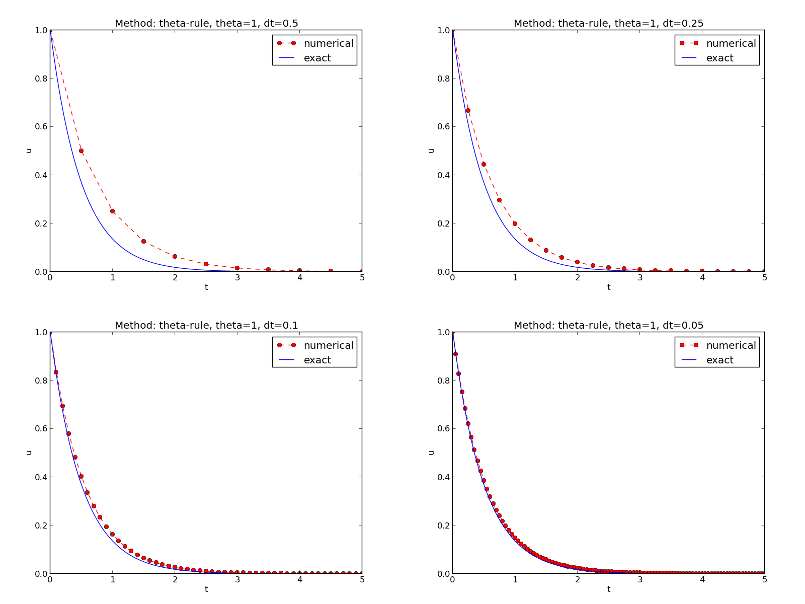
Illustration of the Backward Euler method for four time step values
Ideally, the script should be scalable in the sense that it works for any number of \(\Delta t\) values, which is the case for this particular implementation:
import os, sys

# The command line must contain dt values
if len(sys.argv) > 1:
    dt_values = [float(arg) for arg in sys.argv[1:]]
else:
    print 'Usage: %s dt1 dt2 dt3 ...';  sys.exit(1)  # abort

# Fixed physical parameters
I = 1
a = 2
T = 5

# Run module file as a stand-alone application
cmd = 'python dc_mod.py --I %g --a %g --makeplot --T %g' % \
      (I, a, T)
dt_values_str = ' '.join([str(v) for v in dt_values])
cmd += ' --dt %s' % dt_values_str
print cmd
failure = os.system(cmd)
if failure:
    print 'Command failed:', cmd; sys.exit(1)

# Combine images into rows with 2 plots in each row
combine_image_commands = []
for method in 'BE', 'CN', 'FE':
    imagefiles = ' '.join(['%s_%s.pdf' % (method, dt)
                           for dt in dt_values])
    combine_image_commands.append(
        'montage -background white -geometry 100%' + \
        ' -tile 2x %s %s.png' % (imagefiles, method))
    combine_image_commands.append(
        'convert -trim %s.png %s.png' % (method, method))
    combine_image_commands.append(
        'pdftk %s output tmp.pdf' % imagefiles)
    num_rows = int(round(len(dt_values)/2.0))
    combine_image_commands.append(
        'pdfnup --nup 2x%d tmp.pdf' % num_rows)
    combine_image_commands.append(
        'pdfcrop tmp-nup.pdf')
    combine_image_commands.append(
        'mv -f tmp-nup-crop.pdf %s.pdf;'
        'rm -f tmp.pdf tmp-nup.pdf' % method)
    imagefiles = ' '.join(['%s_%s.png' % (method, dt)
                           for dt in dt_values])

for cmd in combine_image_commands:
    print cmd
    failure = os.system(cmd)
    if failure:
        print 'Command failed:', cmd; sys.exit(1)

# Remove the files generated by dc_mod.py
from glob import glob
filenames = glob('*_*.png') + glob('*_*.pdf') + glob('*_*.eps')  +\
            glob('tmp*.pdf')
for filename in filenames:
    os.remove(filename)
This file is available as experiments/dc_exper0.py.
We may comment upon many useful constructs in this script:
- [float(arg) for arg in sys.argv[1:]] builds a list of real numbers from all the command-line arguments.
- failure = os.system(cmd) runs an operating system command, e.g., another program. The execution successful only if failure is zero.
- Unsuccessful execution usually makes it meaningless to continue the program, and therefore we abort the program with sys.exit(1). Any argument different from 0 signifies that our program stopped with a failure.
- ['%s_%s.png' % (method, dt) for dt in dt_values] builds a list of filenames from a list of numbers (dt_values).
- All montage, pdftk, pdfnup, and mv commands for creating composite figures are stored in a list and later executed in a loop.
- glob('*_*.png') returns a list of the names of all files in the current folder where the filename matches the Unix wildcard notation *_*.png (meaning “any text, underscore, any text, and then .png”).
- os.remove(filename) removes the file with name filename.
Interpreting output from other programs
Programs that run other programs, like dc_exper0.py does, will often need to interpret output from the other programs. Let us demonstrate how this is done in Python by extracting the relations between \(\theta\), \(\Delta t\), and the error \(E\) as written to the terminal window by the dc_mod.py program, which is being executed by dc_exper0.py. We will
- read the output from the dc_mod.py program
- interpret this output and store the \(E\) values in arrays for each \(\theta\) value
- plot \(E\) versus \(\Delta t\), for each \(\theta\), in a log-log plot
The simple os.system(cmd) call does not allow us to read the output from running cmd. Instead we need to invoke a bit more involved procedure:
from subprocess import Popen, PIPE, STDOUT
p = Popen(cmd, shell=True, stdout=PIPE, stderr=STDOUT)
output, dummy = p.communicate()
failure = p.returncode
if failure:
    print 'Command failed:', cmd; sys.exit(1)
The command stored in cmd is run and all text that is written to the standard output and the standard error is available in the string output. The text in output is what appeared in the terminal window while running cmd.
Our next task is to run through the output string, line by line, and if the current line prints \(\theta\), \(\Delta t\), and \(E\), we split the line into these three pieces and store the data. The chosen storage structure is a dictionary errors with keys dt to hold the \(\Delta t\) values, and three \(\theta\) keys to hold the corresponding \(E\) values. The relevant code lines are
errors = {'dt': dt_values, 1: [], 0: [], 0.5: []}
for line in output.splitlines():
    words = line.split()
    if words[0] in ('0.0', '0.5', '1.0'):  # line with E?
        # typical line: 0.0   1.25:    7.463E+00
        theta = float(words[0])
        E = float(words[2])
        errors[theta].append(E)
Note that we do not bother to store the \(\Delta t\) values as we read them from output, because we already have these values in the dt_values list.
We are now ready to plot \(E\) versus \(\Delta t\) for \(\theta=0,0.5,1\):
import matplotlib.pyplot as plt
#import scitools.std as plt
plt.loglog(errors['dt'], errors[0], 'ro-')
plt.hold('on')  # MATLAB style...
plt.loglog(errors['dt'], errors[0.5], 'b+-')
plt.loglog(errors['dt'], errors[1], 'gx-')
plt.legend(['FE', 'CN', 'BE'], loc='upper left')
plt.xlabel('log(time step)')
plt.ylabel('log(error)')
plt.title('Error vs time step')
plt.savefig('error_BE_CN_FE.png')
plt.savefig('error_BE_CN_FE.pdf')
Plots occasionally need some manual adjustments. Here, the axis of the log-log plot look nicer if we adapt them strictly to the data, see Figure Default plot (left) and manually adjusted plot (right). To this end, we need to compute \(\min E\) and \(\max E\), and later specify the extent of the axes:
errors = {'dt': dt_values, 1: [], 0: [], 0.5: []}
min_E = 1E+20; max_E = -min_E  # keep track of min/max E for axis
for line in output.splitlines():
    ...
        ...
        min_E = min(min_E, E);  max_E = max(max_E, E)

import matplotlib.pyplot as plt
plt.loglog(errors['dt'], errors[0], 'ro-')
...
plt.axis([min(dt_values), max(dt_values), min_E, max_E])
...
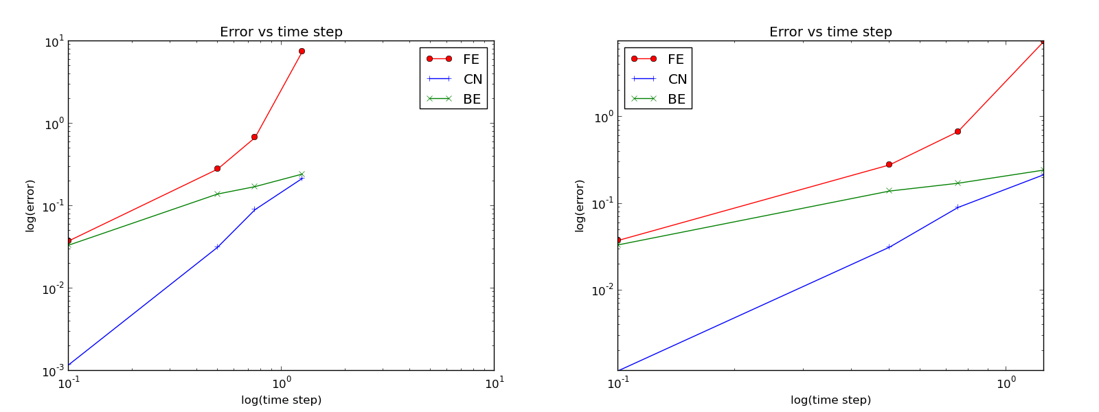
Default plot (left) and manually adjusted plot (right)
The complete program, incorporating the code snippets above, is found in experiments/dc_exper1.py. This program can hopefully be reused in a number of other occasions where one needs to run experiments, extract data from the output of programs, make plots, and combine several plots in a figure file.
Making a report
The results of running computer experiments are best documented in a little report containing the problem to be solved, key code segments, and the plots from a series of experiments. At least the part of the report containing the plots should be automatically generated by the script that performs the set of experiments, because in that script we know exactly which input data that were used to generate a specific plot, thereby ensuring that each figure is connected to the right data. Take a look at an example to see what we have in mind.
Plain HTML
Scientific reports can be written in a variety of formats. Here we begin with the HTML format which allows efficient browsing of all the experiments in any web browser. An extended version of the dc_exper1.py from the last section, called dc_exper1_html.py, adds code at the end for creating an HTML file with a summary, a section on the mathematical problem, a section on the numerical method, a section on the solver function implementing the method, and a section with subsections containing figures that shows the results of experiments where \(\Delta t\) is varied for \(\theta=0,0.5,1\). The mentioned Python file contains all the details for writing this HTML report.
HTML with MathJax
Scientific reports usually need mathematical formulas and hence mathematical typesetting. In plain HTML, as used in the dc_exper1_html.py file, we have to use just the keyboard characters to write mathematics. However, there is an extension to HTML, called MathJax, that allows formulas and equations to be typeset with LaTeX syntax and nicely rendered in web browsers, see Figure Report in HTML format with MathJax. A relatively small subset of LaTeX environments is supported, but the syntax for formulas is quite rich. Inline formulas are look like \( u'=-au \) while equations are surrounded by $$ signs. Inside such signs, one can use \[ u'=-au \] for unnumbered equations, or \begin{equation} and \end{equation} surrounding u'=-au for numbered equations, or \begin{align} and \end{align} for multiple aligned equations, with (align) or without (align*) numbers and labels.
The file dc_exper1_mathjax.py contains all the details for turning the previous plain HTML report into web pages with nicely typeset mathematics.
Report in HTML format with MathJax
LaTeX
The de facto language for mathematical typesetting and scientific report writing is LaTeX, see Figure Report in PDF format generated from LaTeX source for an example. A number of very sophisticated packages have been added to the language over a period of three decades, allowing very fine-tuned layout and typesetting. For output in the PDF format, LaTeX is the definite choice when it comes to quality. The LaTeX language used to write the reports has typically a lot of commands involving backslashes and braces. For output on the web, using HTML (and not the PDF directly in the browser window), LaTeX struggles with delivering high quality typesetting. Other tools, especially Sphinx, gives better results and can also produce nice-looking PDFs. The file dc_exper1_latex.py shows how to generate the LaTeX source from a program.
Report in PDF format generated from LaTeX source
Sphinx
Sphinx is a typesetting language with similarities to HTML and LaTeX, but with much less tagging. It has recently become very popular for software documentation and mathematical reports. Sphinx can utilize LaTeX (via MathJax or PNG images) for mathematical formulas and equations. Unfortunately, the subset of LaTeX mathematics supported is less than in full MathJax (in particular, numbering of multiple equations in an align type environment is not supported). The Sphinx syntax is an extension of the reStructuredText language. An attractive feature of Sphinx is its rich support for fancy layout of web pages. In particular, Sphinx can easily be combined with various layout themes that give a certain look and feel to the web site and that offers table of contents, navigation, and search facilities, see Figure Report in HTML format generated from Sphinx source.
Report in HTML format generated from Sphinx source
Markdown
A recently popular format for easy writing of web pages is Markdown. Text is written very much like one would do in email, using spacing and special characters to naturally format the code instead of heavily tagging the text as in LaTeX and HTML. With the tool Pandoc one can go from Markdown to a variety of formats. HTML is a common output format, but LaTeX, epub, XML, OpenOffice, MediaWiki, and MS Word are some other possibilities.
Wiki formats
A range of wiki formats are popular for creating notes on the web, especially documents which allow groups of people to edit and evolve the content. Apart from MediaWiki (the wiki format used for Wikipedia), wiki formats have no support for mathematical typesetting and also limited tools for displaying computer code in nice ways. Wiki formats are therefore less suitable for scientific reports compared to the other formats mentioned here.
Doconce
Since it is difficult to choose the right tool or format for writing a scientific report, it is advantageous to write the content in a format that easily can be translated to LaTeX, HTML, Sphinx, Markdown, and wikis. Doconce is such a tool. It is similar to Pandoc, but offers some special convenient features for writing about mathematics and programming. The tagging is modest, somewhere between LaTeX and Markdown. The program dc_exper_do.py demonstrates how to generate (and write) Doconce code for a report.
Worked example
The HTML, LaTeX (PDF), Sphinx, and Doconce formats for the scientific report whose content is outlined above, are exemplified with source codes and results at the web pages associated with this teaching material.
Publishing a complete project
A report documenting scientific investigations should be accompanied by all the software and data used for the investigations so that others have a possibility to redo the work and assess the qualify of the results. This possibility is important for reproducible research and hence reaching reliable scientific conclusions.
One way of documenting a complete project is to make a folder tree with all relevant files. Preferably, the tree is published at some project hosting site like Bitbucket, GitHub, or Googlecode so that others can download it as a tarfile, zipfile, or clone the files directly using a version control system like Mercurial or Git. For the investigations outlined in the section Making a report, we can create a folder tree with files
src/dc_mod.py
setup.py
doc/src/dc_exper1_mathjax.py
doc/src/make_report.sh
doc/src/run.sh
doc/pub/report.html
The src directory holds source code (modules) to be reused in other project, the setup.py builds and installs such software, the doc directory contains the documentation, with src for the source of the documentation and pub for ready-made, published documentation. The run.sh file is a simple Bash script listing the python command we used to run dc_exper1_mathjax.py to generate the experiments and report documented in the final published report.html file.
Exercises (1)
Exercise 1: Experiment with integer division
Explain what happens in the following computations, where some are (mathematically) unexpected:
>>> dt = 3
>>> T = 8
>>> N = T/dt
>>> N
2
>>> theta = 1; a = 1
>>> (1 - (1-theta)*a*dt)/(1 + theta*dt*a)
0
Filename: pyproblems.txt.
Exercise 2: Experiment with wrong computations
Consider the solver function in the dc_v1.py and the following call:
u, t = solver(I=1, a=1, T=7, dt=2, theta=1)
The output becomes
t= 0.000 u=1
t= 2.000 u=0
t= 4.000 u=0
t= 6.000 u=0
Print out the result of all intermediate computations and use type(v) to see the object type of the result stored in v. Examine the intermediate calculations and explain why u is wrong and why we compute up to \(t=6\) only even though we specified \(T=7\). Filename: dc_v1_err.py.
Exercise 3: Implement specialized functions
Implement a specialized Python function ForwardEuler that solves the problem \(u'=-au\), \(u(0)=I\), using the Forward Euler method. Do not reimplement the solution algorithm, but let the ForwardEuler function call the solver function. Import this latter function from the module dc_mod. Also make similar functions BackwardEuler and CrankNicolson. Filename: dc_FE_BE_CN.py.
Exercise 4: Plot the error function
Solve the problem \(u'=-au\), \(u(0)=I\), using the Forward Euler, Backward Euler, and Crank-Nicolson schemes. For each scheme, plot the error function \(e_n = u_{\small\mbox{e}}(t_n)-u^n\) for \(\Delta t\), \(\frac{1}{4}\Delta t\), and \(\frac{1}{8}\Delta t\), where \(u_{\small\mbox{e}}\) is the exact solution of the ODE and \(u^n\) is the numerical solution at mesh point \(t_n\). Filename: decay_plot_error.py.
Exercise 5: Compare methods for a give time mesh
Make a program that imports the solver function from the dc_mod module and offers a function compare(dt, I, a) for comparing, in a plot, the methods corresponding to \(\theta=0,0.5,1\) and the exact solution. This plot shows the accuracy of the methods for a given time mesh. Read input data for the problem from the command line using appropriate functions in the dc_mod module (the --dt option for giving several time step values can be reused: just use the first time step value for the computations). Filename: decay_compare_theta.py.
Exercise 6: Change formatting of numbers and debug
The dc_memsave.py program writes the time values and solution values to a file which looks like
0.0000000000000000E+00  1.0000000000000000E+00
2.0000000000000001E-01  8.3333333333333337E-01
4.0000000000000002E-01  6.9444444444444453E-01
6.0000000000000009E-01  5.7870370370370383E-01
8.0000000000000004E-01  4.8225308641975323E-01
1.0000000000000000E+00  4.0187757201646102E-01
1.2000000000000000E+00  3.3489797668038418E-01
1.3999999999999999E+00  2.7908164723365347E-01
Modify the file output such that it looks like
0.000  1.00000
0.200  0.83333
0.400  0.69444
0.600  0.57870
0.800  0.48225
1.000  0.40188
1.200  0.33490
1.400  0.27908
Run
Terminal> python decay8_v2.py --T 10 --theta 1 --dt 0.2 --makeplot
The program just prints Bug in the implementation! and does not show the plot. What went wrong? Filename: dc_memsave_v2.py.
Exercise 7: Write a doctest
Type in the following program and equip the roots function with a doctest:
import sys
# This sqrt(x) returns real if x>0 and complex if x<0
from numpy.lib.scimath import sqrt

def roots(a, b, c):
    """
    Return the roots of the quadratic polynomial
    p(x) = a*x**2 + b*x + c.

    The roots are real or complex objects.
    """
    q = b**2 - 4*a*c
    r1 = (-b + sqrt(q))/(2*a)
    r2 = (-b - sqrt(q))/(2*a)
    return r1, r2

a, b, c = [float(arg) for arg in sys.argv[1:]]
print roots(a, b, c)
Make sure to test both real and complex roots. Write out numbers with 14 digits or less. Filename: doctest_roots.py.
Exercise 8: Write a nose test
Make a nose test for the roots function in Exercise 7: Write a doctest. Filename: test_roots.py.
Exercise 9: Make a module
Let
Make a Python module q_module containing two functions q(t) and dqdt(t) for computing \(q(t)\) and \(q'(t)\), respectively. Perform a from numpy import * in this module. Import q and dqdt in another file using the “star import” construction from q_module import *. All objects available in this file is given by dir(). Print dir() and len(dir()). Then change the import of numpy in q_module.py to import numpy as np. What is the effect of this import on the number of objects in dir() in a file that does from q_module import *?
Filename: q_module.py.
Exercise 10: Make use of a class implementation
We want to solve the exponential decay problem \(u'=-au\), \(u(0)=I\), for several \(\Delta t\) values and \(\theta=0,0.5,1\). For each \(\Delta t\) value, we want to make a plot where the three solutions corresponding to \(\theta=0,0.5,1\) appear along with the exact solution. Write a function experiment to accomplish this. The function should import the classes Problem, Solver, and Visualizer from the decay_class1 module and make use of these. A new command-line option --dt_values must be added to allow the user to specify the \(\Delta t\) values on the command line (the options --dt and --theta have then no effect when running the experiment function). Note that the classes in the decay_class1 module should not be modified.
Filename: dc_class_exper.py.
Analysis of the \(\theta\)-rule for a decay ODE
We address the ODE for exponential decay,
where \(a\) and \(I\) are given constants. This problem is solved by the \(\theta\)-rule finite difference scheme, resulting in the recursive equations
for the numerical solution \(u^{n+1}\), which approximates the exact solution \(u_{\small\mbox{e}}\) at time point \(t_{n+1}\). For constant mesh spacing, which we assume here, \(t_{n+1}=(n+1)\Delta t\).
Discouraging numerical solutions
Choosing \(I=1\), \(a=2\), and running experiments with \(\theta =1,0.5, 0\) for \(\Delta t=1.25, 0.75, 0.5, 0.1\), gives the results in Figures Backward Euler, Crank-Nicolson, and Forward Euler.
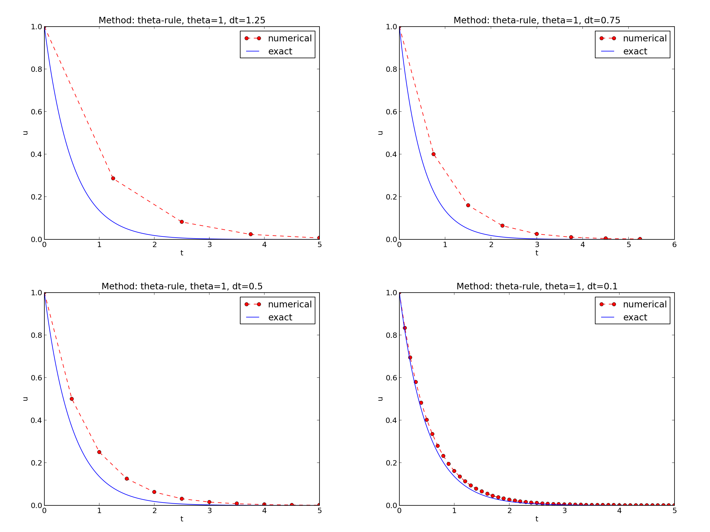
Backward Euler
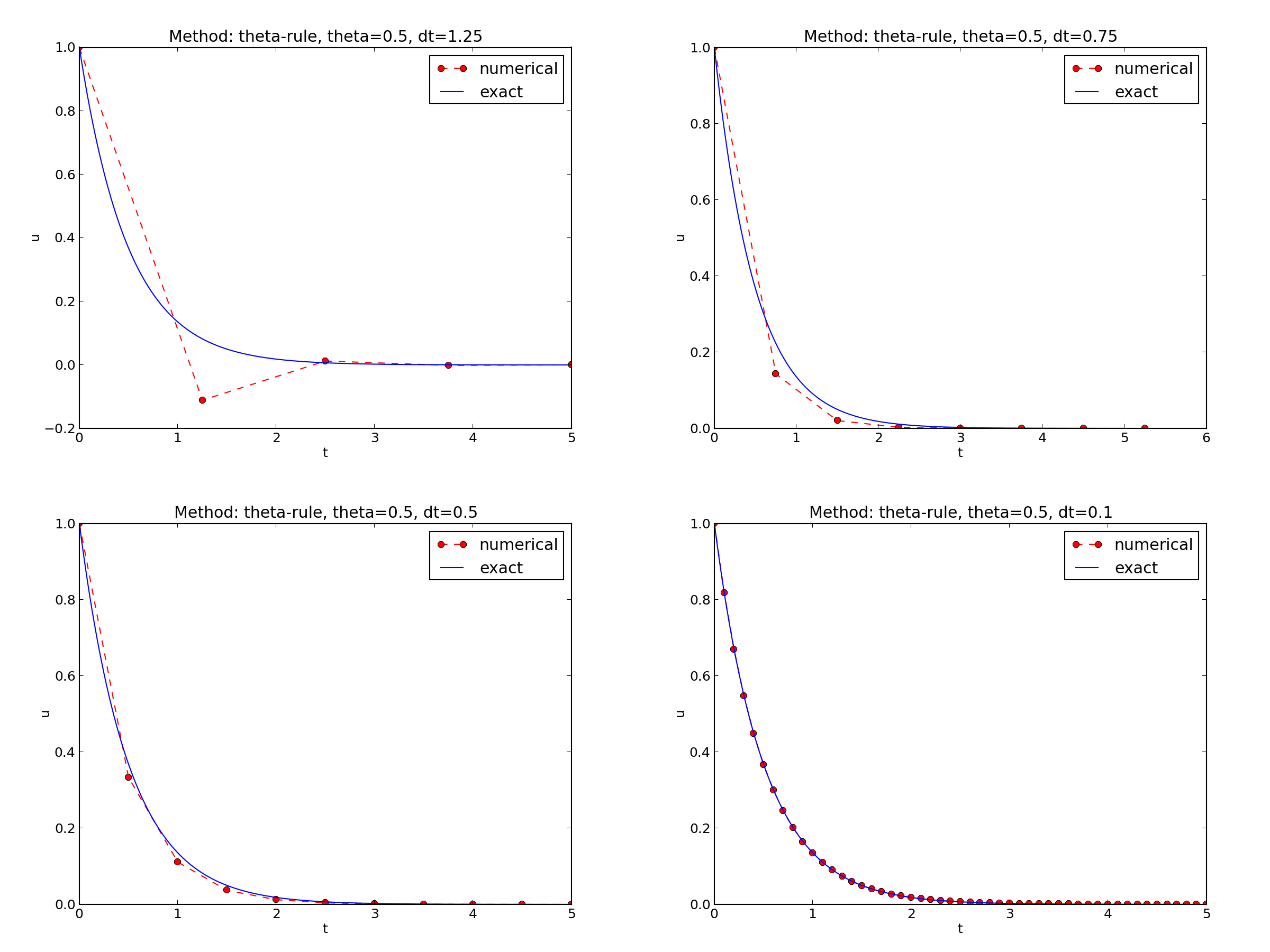
Crank-Nicolson
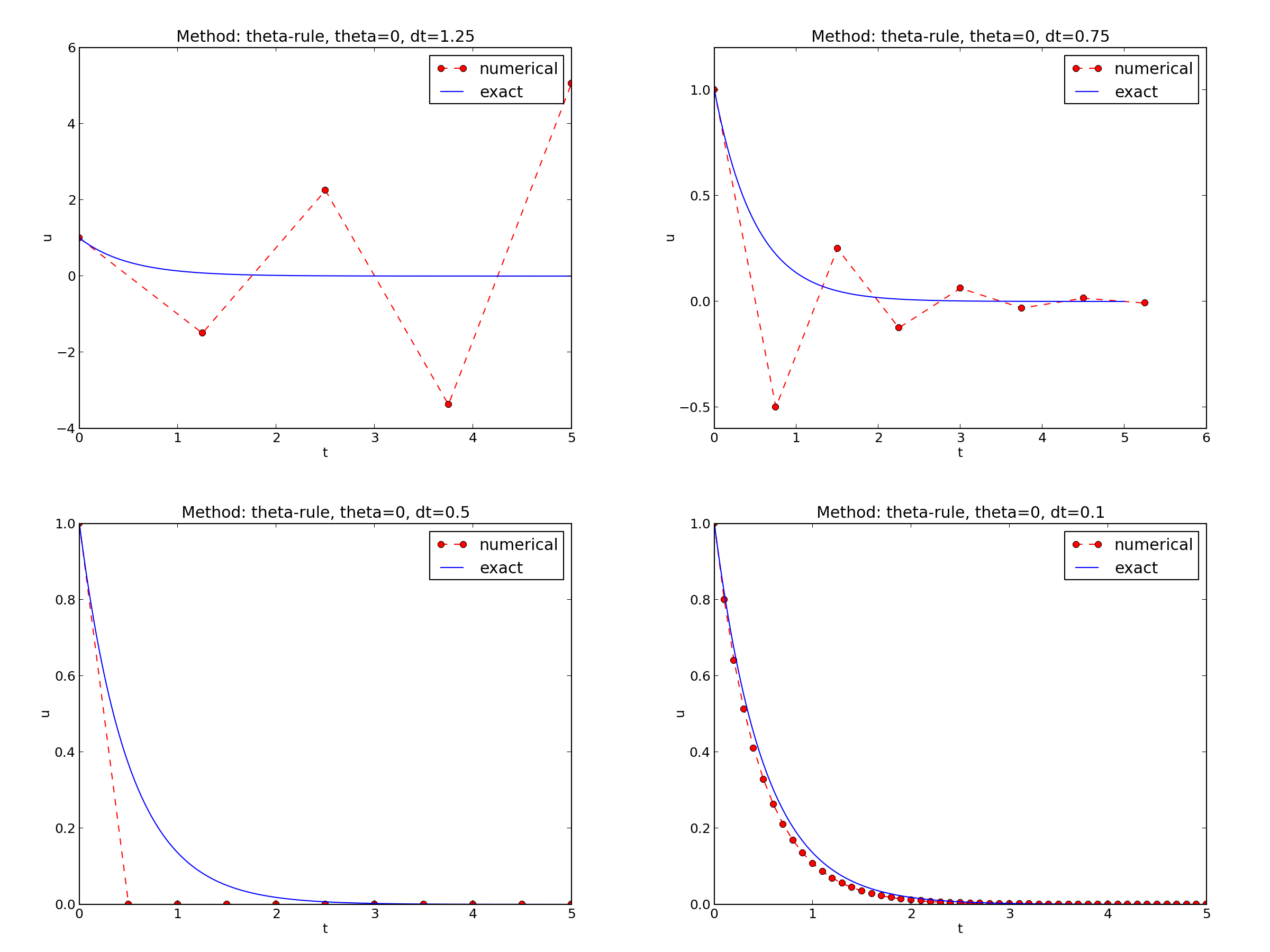
Forward Euler
The characteristics of the displayed curves can be summarized as follows:
- The Backward Euler scheme always give a monotone solution, lying above the exact curve.
- The Crank-Nicolson scheme gives the most accurate results, but for \(\Delta t=1.25\) the solution oscillates.
- The Forward Euler scheme gives a growing, oscillating solution for \(\Delta t=1.25\); a decaying, oscillating solution for \(\Delta t=0.75\); a strange solution \(u^n=0\) for \(n\geq 1\) when \(\Delta t=0.5\); and a solution seemingly as accurate as the one by the Backward Euler scheme for \(\Delta t = 0.1\), but the curve lies below the exact solution.
Since the exact solution of our model problem is a monotone function, \(u(t)=Ie^{-at}\), some of these qualitatively wrong results are indeed alarming!
Experimental investigation of oscillatory solutions
We may ask the question: Under what circumstances, i.e., values of the input data \(I\), \(a\), and \(\Delta t\) will the Forward Euler and Crank-Nicolson schemes result in undesired oscillatory solutions?
We may set up an experiment where we loop over values of \(I\), \(a\), and \(\Delta t\). For each experiment, we flag the solution as oscillatory if
for some value of \(n\), since we expect \(u^n\) to decay with \(n\), but oscillations make \(u\) increase over a time step. We will quickly see that oscillations are independent of \(I\), but do depend on \(a\) and \(\Delta t\). Therefore, we introduce a two-dimensional function \(B(a,\Delta t)\) which is 1 if oscillations occur and 0 otherwise. We can visualize \(B\) as a contour plot (lines for which \(B=\hbox{const}\)). The contour \(B=0.5\) will correspond to the borderline between oscillatory regions with \(B=1\) and monotone regions with \(B=0\) in the \(a-\Delta t\) plane.
The \(B\) function is defined at discrete \(a\) and \(\Delta t\) values. Say we have given \(P\) $a$ values, \(a_0,\ldots,a_{P-1}\), and \(Q\) $Delta t$ values, \(\Delta t_0,\ldots,\Delta t_{Q-1}\). These \(a_i\) and \(\Delta t_j\) values, \(i=0,\ldots,P-1\), \(j=0,\ldots,Q-1\), form a rectangular mesh of \(P\times Q\) points in the plane. At each point \((a_i, \Delta t_j)\), we associate the corresponding value of \(B(a_i,\Delta t_j)\), denoted \(B_{ij}\). The \(B_{ij}\) values are naturally stored in a two-dimensional array. Both Matplotlib and SciTools can create a plot of the contour line \(B_{ij}=0.5\) dividing the oscillatory and monotone regions. The file dc_osc_regions.py contains all nuts and bolts to produce the \(B=0.5\) line in Figures Forward Euler scheme: oscillatory solutions occur for points above the curve and Crank-Nicolson scheme: oscillatory solutions occur for points above the curve. The oscillatory region is above this line.
from dc_mod import solver
import numpy as np
import scitools.std as st

def non_physical_behavior(I, a, T, dt, theta):
    """
    Given lists/arrays a and dt, and numbers I, dt, and theta,
    make a two-dimensional contour line B=0.5, where B=1>0.5
    means oscillatory (unstable) solution, and B=0<0.5 means
    monotone solution of u'=-au.
    """
    a = np.asarray(a); dt = np.asarray(dt)  # must be arrays
    B = np.zeros((len(a), len(dt)))         # results
    for i in range(len(a)):
        for j in range(len(dt)):
            u, t = solver(I, a[i], T, dt[j], theta)
            # Does u have the right monotone decay properties?
            correct_qualitative_behavior = True
            for n in range(1, len(u)):
                if u[n] > u[n-1]:  # Not decaying?
                    correct_qualitative_behavior = False
                    break  # Jump out of loop
            B[i,j] = float(correct_qualitative_behavior)
    a_, dt_ = st.ndgrid(a, dt)  # make mesh of a and dt values
    st.contour(a_, dt_, B, 1)
    st.grid('on')
    st.title('theta=%g' % theta)
    st.xlabel('a'); st.ylabel('dt')
    st.savefig('osc_region_theta_%s.png' % theta)
    st.savefig('osc_region_theta_%s.eps' % theta)

non_physical_behavior(
    I=1,
    a=np.linspace(0.01, 4, 22),
    dt=np.linspace(0.01, 4, 22),
    T=6,
    theta=0.5)
Forward Euler scheme: oscillatory solutions occur for points above the curve
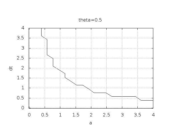
Crank-Nicolson scheme: oscillatory solutions occur for points above the curve
By looking at the curves in the figures one may guess that \(a\Delta t\) must be less than a critical limit to avoid the undesired oscillations. This limit seems to be about 2 for Crank-Nicolson and 1 for Forward Euler. We shall now establish a mathematical analysis of the discrete model that can explain the observations in our numerical experiments.
Exact numerical solution
Starting with \(u^0=I\), the simple recursion (29) can be applied repeatedly \(n\) times, with the result that
Difference equations where all terms are linear in \(u^{n+1}\), \(u^n\), and maybe \(u^{n-1}\), \(u^{n-2}\), etc., are called homogeneous, linear difference equations, and their solutions are generally of the form \(u^n=A^n\). Inserting this expression and dividing by \(A^{n+1}\) gives a polynomial equation in \(A\). In the present case we get
This is a solution technique of wider applicability than repeated use of the recursion (29).
Regardless of the solution approach, we have obtained a formula for \(u^n\). This formula can explain everything what we see in the figures above, but it also gives us a more general insight into accuracy and stability properties of the three schemes.
Stability
Since \(u^n\) is a factor
raised to an integer power (\(n\)), we realize that \(A<0\) will for odd powers imply \(u^n<0\) and for even power result in \(u^n>0\), i.e., a solution that oscillates between the mesh points. We have that \(A<0\) when
Since \(A>0\) is a requirement for having a numerical solution with the same basic property (monotonicity) as the exact solution, we may say that \(A>0\) is a stability criterion. Expressed in terms of \(\Delta t\) the stability criterion reads
The Backward Euler scheme is always stable (since \(A<0\) is impossible), while non-oscillating solutions for Forward Euler and Crank-Nicolson demand \(\Delta t\leq 1/a\) and \(\Delta t\leq 2/a\), respectively. The relation between \(\Delta t\) and \(a\) look reasonable: a smaller \(a\) means faster decay and hence a need for smaller time steps.
Looking at Figure Forward Euler, we see that with \(a\Delta t= 2\cdot 1.25=2.5\), \(A=-1.5\), and the solution \(u^n=(-1.5)^n\) oscillates and grows. With \(a\Delta t = 2\cdot 0.75=1.5\), \(A=-0.5\), \(u^n=(-0.5)^n\) decays but oscillates. The peculiar case \(\Delta t = 0.5\), where the Forward Euler scheme produces a solution that is stuck on the \(t\) axis, corresponds to \(A=0\) and therefore \(u^0=I=1\) and \(u^n=0\) for \(n\geq 1\). The decaying oscillations in the Crank-Nicolson scheme for \(\Delta t=1.25\) is easily explained by \(A=-0.25\).
The factor \(A\) is called amplification factor since the solution at a new time level is \(A\) times the solution at the previous time level. For a decay process, we must obviously have \(|A|\leq 1\) for all \(\Delta t\), which is fulfilled for \(\theta \geq 1/2\). Arbitrarily large values of \(u\) can be generated when \(|A|>1\) and \(n\) is large enough. The numerical solution is in such cases totally irrelevant to an ODE modeling decay processes.
Comparing Amplification Factors
After establishing how \(A\) impacts the qualitative features of the solution, we shall now look more into how well the numerical amplification factor approximates the exact one. The exact solution reads \(u(t)=Ie^{-at}\), which can be rewritten as
From this formula we see that the exact amplification factor is
We realize that the exact and numerical amplification factors depend on \(a\) and \(\Delta t\) through the product \(a\Delta t\). Therefore, it is convenient to introduce a symbol for this product, \(p=a\Delta t\), and view \(A\) and \(A_{\small\mbox{e}}\) as functions of \(p\). Figure Comparison of amplification factors shows these functions. Crank-Nicolson is clearly closest to the exact amplification factor, but that method has the unfortunate oscillatory behavior when \(p>2\).
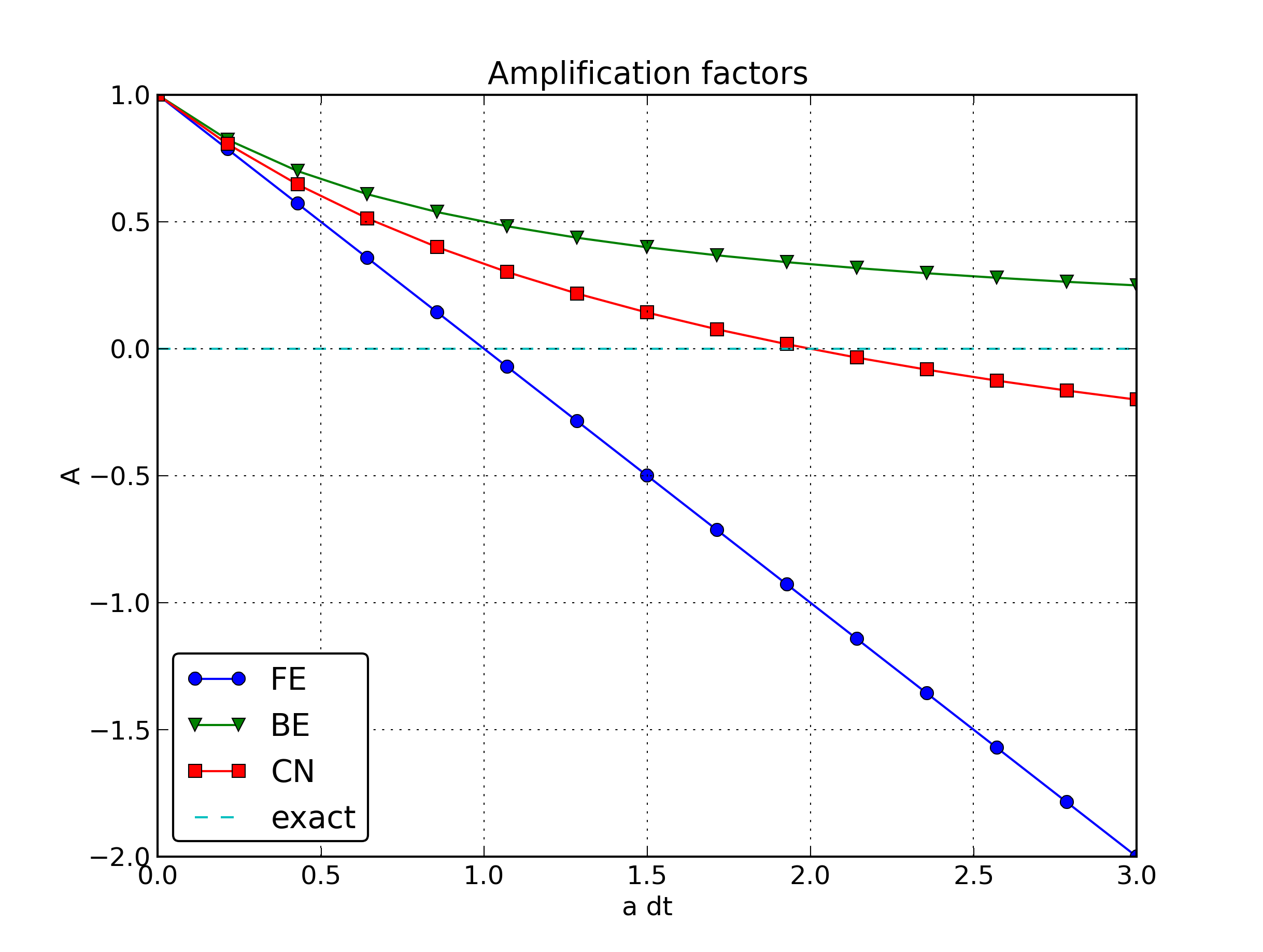
Comparison of amplification factors
Series Expansion of Amplification Factors
As an alternative to the visual understanding inherent in Figure Comparison of amplification factors, there is a strong tradition in numerical analysis to investigate approximation errors when the discretization parameter, here \(\Delta t\), becomes small. In the present case we let \(p\) be our small discretization parameter, and it makes sense to simplify the expressions for \(A\) and \(A_{\small\mbox{e}}\) by using Taylor polynomials around \(p=0\). The Taylor polynomials are accurate for small \(p\) and greatly simplifies the comparison of the analytical expressions since we then can compare polynomials, term by term.
Calculating the Taylor series for \(A_{\small\mbox{e}}\) is easily done by hand, but the three versions of \(A\) for \(\theta=0,1,\frac{1}{2}\) lead to more cumbersome calculations. Nowadays, analytical computations can benefit greatly by symbolic computer algebra software. The Python package sympy represents a powerful computer algebra system, not as sophisticated as the famous Maple and Mathematica systems, but free and very easy to integrate with our numerical computations in Python.
When using sympy, it is convenient to enter the interactive Python mode where we can write expressions and statements and immediately see the results. Here is a simple example. We strongly recommend to use isympy (or ipython) for such interactive sessions, although our typesetting will apply the different prompt >>> (associated with the primitive Python shell that results from writing python in a terminal window).
Let us enter sympy in a Python shell and show how we can find the Taylor series for \(e^{-p}\):
>>> from sympy import *
>>> p = Symbol('p')  # all variables must be declared as Symbols
>>> A_e = exp(-p)
>>>
>>> # First 6 terms of the Taylor series of A_e
>>> A_e.series(p, 6)
1 + (1/2)*p**2 - p - 1/6*p**3 - 1/120*p**5 + (1/24)*p**4 + O(p**6)
Lines with >>> represent input lines and lines without this prompt represents the result of computations. Apart from the order of the powers, the computed formula is easily recognized as the beginning of the Taylor series for \(e^{-p}\).
Let us define the numerical amplification factor where \(p\) and \(\theta\) enter the formula as symbols:
>>> theta = Symbol('theta')
>>> A = (1-(1-theta)*p)/(1+theta*p)
To work with the factor for the Backward Euler scheme we can substitute the value 1 for theta:
>>> A.subs(theta, 1)
1/(1 + p)
Similarly, we can substitute theta by 1/2 for Crank-Nicolson, preferably using an exact rational representation of 1/2 in sympy:
>>> half = Rational(1,2)
>>> A.subs(theta, half)
1/(1 + (1/2)*p)*(1 - 1/2*p)
The Taylor series of the amplification factor for the Crank-Nicolson scheme can be computed as
>>> A.subs(theta, half).series(p, 4)
1 + (1/2)*p**2 - p - 1/4*p**3 + O(p**4)
We are now in a position to compare Taylor series:
>>> FE = A_e.series(p, 4) - A.subs(theta, 0).series(p, 4)
>>> BE = A_e.series(p, 4) - A.subs(theta, 1).series(p, 4)
>>> CN = A_e.series(p, 4) - A.subs(theta, half).series(p, 4)
>>> FE
(1/2)*p**2 - 1/6*p**3 + O(p**4)
>>> BE
-1/2*p**2 + (5/6)*p**3 + O(p**4)
>>> CN
(1/12)*p**3 + O(p**4)
From these expressions we see that the error \(A-A_{\small\mbox{e}}\sim {\cal O}(p^2)\) for the Forward and Backward Euler schemes, while \(A-A_{\small\mbox{e}}\sim {\cal O}(p^3)\) for the Crank-Nicolson scheme. It is the leading order term, i.e., the term of the lowest order (degree), that is of interest, because as \(p\rightarrow 0\), this term is (much) bigger than the higher-order terms.
Now, \(a\) is a given parameter in the problem, while \(\Delta t\) is what we can vary. One therefore usually writes the error expressions in terms \(\Delta t\). When then have
What is the significance of this result? If we halve \(\Delta t\), the error in amplification factor at a time level will be reduced by a factor of 4 in the Forward and Backward Euler schemes, and by a factor of 8 in the Crank-Nicolson scheme. That is, as we reduce \(\Delta t\) to obtain more accurate results, the Crank-Nicolson scheme reduces the error more efficiently than the other schemes.
Local error
(max/infinity norm etc). Both errors can be investigated analytically.]
Analytical comparison of schemes
An alternative comparison of the schemes is to look at the ratio \(A/A_{\small\mbox{e}}\), or the error \(1-A/A_{\small\mbox{e}}\) in this ratio:
>>> FE = 1 - (A.subs(theta, 0)/A_e).series(p, 4)
>>> BE = 1 - (A.subs(theta, 1)/A_e).series(p, 4)
>>> CN = 1 - (A.subs(theta, half)/A_e).series(p, 4)
>>> FE
(1/2)*p**2 + (1/3)*p**3 + O(p**4)
>>> BE
-1/2*p**2 + (1/3)*p**3 + O(p**4)
>>> CN
(1/12)*p**3 + O(p**4)
The leading-order terms have the same powers as in the analysis of \(A-A_{\small\mbox{e}}\).
The real (global) error at a point
The error in the amplification factor reflects the error when progressing from time level \(t_n\) to \(t_{n-1}\). To investigate the real error at a point, known as the global error, we look at \(u^n-u_{\small\mbox{e}}(t_n)\) for some \(n\) and Taylor expand the mathematical expressions as functions of \(p=a\Delta t\):
>>> n = Symbol('n')
>>> u_e = exp(-p*n)
>>> u_n = A**n
>>> FE = u_e.series(p, 4) - u_n.subs(theta, 0).series(p, 4)
>>> BE = u_e.series(p, 4) - u_n.subs(theta, 1).series(p, 4)
>>> CN = u_e.series(p, 4) - u_n.subs(theta, half).series(p, 4)
>>> FE
(1/2)*n*p**2 - 1/2*n**2*p**3 + (1/3)*n*p**3 + O(p**4)
>>> BE
(1/2)*n**2*p**3 - 1/2*n*p**2 + (1/3)*n*p**3 + O(p**4)
>>> CN
(1/12)*n*p**3 + O(p**4)
For a fixed time \(t\), the parameter \(n\) in these expressions increases as \(p\rightarrow 0\) since \(t=n\Delta t\). That is, \(n=t/\Delta t\), and the leading-order error terms therefore become \(\frac{1}{2}na^2\Delta t^2 = \frac{1}{2}ta^2t\Delta t\) for the Forward and Backward Euler scheme, and \(\frac{1}{12}na^3\Delta t^3 = \frac{1}{12}ta^3\Delta t^2\) for the Crank-Nicolson scheme. The global error is therefore of second order in \(\Delta t\) for the latter scheme and first order for the former schemes.
Integrated errors
The formulas for various error measures have so far measured the error at one time point. Many prefer to use the error integrated over the whole time interval of interest: \([0,T]\). An immediate practical problem arises, however, since the numerical solution is only known at the mesh points, while an integration will need this solution also at the points between the mesh points. Let \(\tilde u\) be a continuous representation of the numerical solution, usually obtained by drawing straight lines between the values at the mesh points. Then a common measure of the global error is the so-called \(L^2\) error:
A family of such measures is the \(L^p\) errors, defined as
For \(p=1\) we just take the absolute value of the integrand.
Strictly speaking, it is questionable in a finite difference method to introduce an additional approximation in the error measure, namely how \(\tilde u\) varies between the mesh points. Some may argue and say that the numerical solution is defined at the mesh points only and that we should approximate the integrals above by numerical methods involving the integrand at just the mesh points. The numerical integration method also represents an approximation, but a discrete integration procedure is consistent with having only discrete values of the integrand.
For uniformly distributed mesh points we have the well-known Trapezoidal rule,
In case the mesh points are arbitrarily spaced, we have an immediate generalization in terms of the sum of the various trapezoids:
A simpler approximation is to use rectangles whose heights are determined by the left (or right) value in each interval:
With uniformly distributed mesh points we get the simplification
Suppose that in a program the \(u^k\) values are available as elements in the array u, while the \({u_{\small\mbox{e}}}(k\Delta t)\) values are available as elements in the array u_e. The formula (35) can then be calculated as follows by array arithmetics in Python:
E2 = sqrt(dt*sum((u_e - u)**2))
This is exactly the “array formula” that popped up in the section Computing the numerical error.
Integrated error measures sum up the contributions from each mesh point, so we must expect the global error to be larger than the local error. Roughly speaking, if \(|u_{\small\mbox{e}}(t_n) - u^n|\sim ta^{r+1}\Delta t^r\), we have
since \(t=i\Delta t\), \(\sum_{i=0}^N i^2\approx \frac{1}{3}N^3\), and \(N=T/Delta t\).
Exercises (2)
Exercise 11: Explore the \(\theta\)-rule for exponential growth
Solve the ODE \(u'=-au\) with \(a<0\) such that the ODE models exponential growth. Run experiments with \(\theta\) and \(\Delta t\) using the dc_exper1.py code modified to your needs. Are there any numerical artifacts? Filename: growth_exper1.py.
Exercise 12: Summarize investigations in a report
Write a scientific report about the findings in Exercise 11: Explore the -rule for exponential growth. You can use examples from the section Making a report to see how various formats can be used for scientific reports. Filename: growth_analysis.pdf.
Exercise 13: Plot amplification factors for exponential growth
Modify the dc_ampf_plot.py code to visualize the amplification factors for \(\theta =0, 0.5, 1\) and the exact amplification factor in case of exponential growth as in Exercise 11: Explore the -rule for exponential growth. Explain the artifacts seen in Exercise 11: Explore the -rule for exponential growth. Filename: growth_ampf_plot.py.
Model extensions
It is time to consider generalizations of the simple decay model \(u=-au\), where \(a\) is constant, and also to look at other numerical solution methods.
Generalization: including a variable coefficient
In the ODE for decay, \(u'=-au\), we now consider the case where \(a\) depends on time:
A Forward Euler scheme consist of evaluating (36) at \(t=t_n\) and approximating the derivative with a forward difference \([D^+_t u]^n\):
The Backward Euler scheme becomes
The Crank-Nicolson method builds on sampling the ODE at \(t_{n+\frac{1}{2}}\). We can evaluate \(a\) at \(t_{n+\frac{1}{2}}\) and use an average for \(u\) at times \(t_n\) and \(t_{n+1}\):
Alternatively, we can use an average for the product \(au\):
The \(\theta\)-rule unifies the three mentioned schemes. Either with \(a\) evaluated at \(t_{n+\theta}\),
or using a weighted average for the product \(au\),
With the finite difference operator notation the Forward Euler and Backward Euler schemes can be summarized as
The Crank-Nicolson and \(\theta\) schemes depend on whether we evaluate \(a\) at the sample point for the ODE or if we use an average. The various versions are written as
Generalization: including a source term
A further extension of the model ODE is to include a source term \(b(t)\):
Schemes
The time point where we sample the ODE determines where \(b(t)\) is evaluated. For the Crank-Nicolson scheme and the \(\theta\)-rule we have a choice of whether to evaluate \(a(t)\) and \(b(t)\) at the correct point or use an average. The chosen strategy becomes particularly clear if we write up the schemes in the operator notation:
Implementation of the generalized model problem
Deriving the \(\theta\)-rule formula
Writing out the \(\theta\)-rule in (38), using (?) and (?), we get
where \(a^n\) means evaluating \(a\) at \(t=t_n\) and similar for \(a^{n+1}\), \(b^n\), and \(b^{n+1}\). We solve for \(u^{n+1}\):
The Python code
Here is a suitable implementation of (39) where \(a(t)\) and \(b(t)\) are given as Python functions:
def solver(I, a, b, T, dt, theta):
    """
    Solve u'=-a(t)*u + b(t), u(0)=I,
    for t in (0,T] with steps of dt.
    a and b are Python functions of t.
    """
    dt = float(dt)           # avoid integer division
    N = int(round(T/dt))     # no of time intervals
    T = N*dt                 # adjust T to fit time step dt
    u = zeros(N+1)           # array of u[n] values
    t = linspace(0, T, N+1)  # time mesh

    u[0] = I                 # assign initial condition
    for n in range(0, N):    # n=0,1,...,N-1
        u[n+1] = ((1 - dt*(1-theta)*a(t[n]))*u[n] + \
                  dt*(theta*b(t[n+1]) + (1-theta)*b(t[n])))/\
                  (1 + dt*theta*a(t[n+1]))
    return u, t
This function is found in the file dc_vc.py.
Coding of variable coefficients
The solver function shown above demands the arguments a and b to be Python functions of time t, say
def a(t):
    return a_0 if t < tp else k*a_0

def b(t):
    return 1
Here, a(t) has three parameters a0, tp, and k, which must be global variables. A better implementation is to represent a by a class where the parameters are attributes and a special method __call__ evaluates \(a(t)\):
class A:
    def __init__(self, a0=1, k=2):
        self.a0, self.k = a0, k

    def __call__(self, t):
        return self.a0 if t < self.tp else self.k*self.a0

a = A(a0=2, k=1)  # a behaves as a function a(t)
For quick tests it is cumbersome to write a complete function or a class. The lambda function construction in Python is then convenient. For example,
a = lambda t: a_0 if t < tp else k*a_0
is equivalent to the def a(t): definition above. In general,
f = lambda arg1, arg2, ...: expressin
is equivalent to
def f(arg1, arg2, ...):
    return expression
One can use lambda functions directly in calls. Say we want to solve \(u'=-u+1\), \(u(0)=2\):
u, t = solver(2, lambda t: 1, lambda t: 1, T, dt, theta)
A lambda function can appear anywhere where a variable can appear.
Verification via trivial solutions
A very useful partial verification method is to construct a test problem with a very simple solution, usually \(u=\hbox{const}\). Especially the initial debugging of a program code can benefit greatly from such tests, because 1) all relevant numerical methods will exactly reproduce a constant solution, and 2) many of the intermediate calculations are easy to control for a constant \(u\).
The only constant solution for the problem \(u'=-au\) is \(u=0\), but too many bugs can escape from that trivial solution. It is much better to search for a problem where \(u=C=\hbox{const}\neq 0\). Then \(u'=-a(t)u + b(t)\) is more appropriate. With \(u=C\) we can choose any \(a(t)\) and set \(b=a(t)C\) and \(I=C\). An appropriate nose test is
import nose.tools as nt

def test_constant_solution():
    """
    Test problem where u=u_const is the exact solution, to be
    reproduced (to machine precision) by any relevant method.
    """
    def exact_solution(t):
        return u_const

    def a(t):
        return 2.5*(1+t**3)  # can be arbitrary

    def b(t):
        return a(t)*u_const

    u_const = 2.15
    theta = 0.4; I = u_const; dt = 4
    N = 4  # enough with a few steps
    u, t = solver(I=I, a=a, b=b, T=N*dt, dt=dt, theta=theta)
    print u
    u_e = exact_solution(t)
    difference = abs(u_e - u).max()  # max deviation
    nt.assert_almost_equal(difference, 0, places=14)
An interesting question is what type of bugs that will make the computed \(u^n\) to deviate from the exact solution \(C\). Fortunately, the updating formula and the initial condition must be absolutely correct for the test to pass! Any attempt to make a wrong indexing in terms like a(t[n]) or any attempt to introduce an erroneous factor in the formula creates a solution that is different from \(C\).
Verification via manufactured solutions
Following the idea of the previous section, we can choose any formula as the exact solution, insert the formula in the ODE problem and fit the data \(a(t)\), \(b(t)\), and \(I\) to make the chosen formula fulfill the equation. This powerful technique for generating exact solutions is very useful for verification purposes and known as the method of manufactured solutions, often abbreviated MMS.
One common choice of solution is a linear function in the independent variable(s). The rationale behind such a simple variation is that almost any relevant numerical solution method for differential equation problems is able to reproduce the linear function exactly to machine precision (if \(u\) is about unity in size; precision is lost if \(u\) take on large values, see decay:fd2:exer:precision). The linear solution also makes some stronger demands to the numerical method and the implementation than the constant solution used in the section Verification via trivial solutions, at least in more complicated applications. However, the constant solution is often ideal for initial debugging before proceeding with a linear solution.
We choose \(u(t) = ct + d\). We must then have \(d=I\) from the initial condition. Inserting this \(u\) in the ODE results in
Any function \(u=ct+I\) is then a correct solution if we choose
With this \(b(t)\) there are no restrictions on \(a(t)\) and \(c\).
Let us see if such a linear solution obeys the numerical schemes. That is, we must check that \(u^n = ca(t_n)(ct_n+I)\) fits the discrete equations. To this end, it is convenient to compute the action of a difference operator on \(u^n=t_n\):
The difference equation for the Forward Euler scheme
with \(a^n=a(t_n)\), \(b^n=c + a(t_n)(ct_n + I)\), and \(u^n=ct_n + I\) then results in
which is always fulfilled. Similar calculations can be done for the Backward Euler and Crank-Nicolson schemes, or the \(\theta\)-rule for that matter. In all cases, \(u^n=ct_n +I\) is an exact solution of the discrete equations. That is why we should expect that \(u^n - u_{\small\mbox{e}}(t_n) =0\) mathematically and \(|u^n - u_{\small\mbox{e}}(t_n)|\) less than a small number about the machine precision for \(n=0,\ldots,N\).
The following function offers an implementation of this verification test based on a linear exact solution:
def test_linear_solution():
    """
    Test problem where u=c*t+I is the exact solution, to be
    reproduced (to machine precision) by any relevant method.
    """
    def exact_solution(t):
        return c*t + I

    def a(t):
        return t**0.5  # can be arbitrary

    def b(t):
        return c + a(t)*exact_solution(t)

    theta = 0.4; I = 0.1; dt = 0.1; c = -0.5
    T = 4
    N = int(T/dt)  # no of steps
    u, t = solver(I=I, a=a, b=b, T=N*dt, dt=dt, theta=theta)
    u_e = exact_solution(t)
    difference = abs(u_e - u).max()  # max deviation
    print difference
    # No of decimal places for comparison depend on size of c
    nt.assert_almost_equal(difference, 0, places=14)
As in the section Verification via trivial solutions, any error in the updating formula makes this test fail.
Choosing more complicated formulas as the exact solution, say \(\cos(t)\), will not make the numerical and exact solution coincide to machine precision. In such cases, the verification procedure must be based on measuring the convergence rates as exemplified in the section Computing convergence rates. This is possible since one has an exact solution of a problem that the solver can be tested on.
Extension to systems of ODEs
Many ODE models involves more than one unknown function and more than one equation. Here is an example of two unknown functions \(u(t)\) and \(v(t)\) (modeling, e.g., the radioactive decay of two substances):
for constants \(a_u, a_v>0\). Applying the Forward Euler method to each equation results in simple updating formula
However, the Crank-Nicolson or Backward Euler schemes result in a \(2\times 2\) linear system for the new unknowns. The latter schemes gives
and bringing \(u^{n+1}\) as well as \(v^{n+1}\) on the left-hand side results in
which is a system of two coupled, linear, algebraic equations in two unknowns.
General first-order ODEs
We now turn the attention to general, nonlinear ODEs and systems of such ODEs. Many schemes that are often reused for time-discretization of PDEs are listed. We also demonstrate a Python interface to a range of different software for general first-order ODE systems.
Generic form
ODEs are commonly written in the generic form
where \(f(u,t)\) is a prescribed function. As an example, our most general exponential decay model (37) has \(f(u,t)=-a(t)u(t) + b(t)\).
The unknown \(u\) in (41) may either be a scalar function of time \(t\), or a vector valued function of \(t\) in case of a system of ODEs:
In that case, the right-hand side is vector-valued function with \(m\) components,
Actually, any system of ODEs can be written in the form (41), but higher-order ODEs then need auxiliary unknown functions.
The Odespy software
A wide range of the methods and software exist for solving (41). Many of methods are accessible through a unified Python interface offered by the Odespy package. Odespy features simple Python implementations of the most fundamental schemes as well as Python interfaces to several famous packages for solving ODEs: ODEPACK, Vode, rkc.f, rkf45.f, Radau5, as well as the ODE solvers in SciPy, SymPy, and odelab.
The usage of Odespy follows this setup for the ODE \(u'=-au\), \(u(0)=I\), \(t\in (0,T]\), here solved by the famous 4th-order Runge-Kutta method, using \(\Delta t=1\) and \(N=6\) steps:
def f(u, t):
    return -a*u

import odespy
import numpy as np

I = 1; a = 0.5; N = 6; dt = 1
solver = odespy.RK4(f)
solver.set_initial_condition(I)
t_mesh = np.linspace(0, N*dt, N+1)
u, t = solver.solve(t_mesh)
Example: Runge-Kutta methods
Since all solvers have the same interface, modulo different set of parameters to the solvers’ constructors, one can easily make a list of solver objects and run a loop for comparing (a lot of) solvers. The code below, found in complete form in dc_odespy.py, compares the famous Runge-Kutta methods of orders 2, 3, and 4 with the exact solution of the decay equation \(u'=-au\). Since we have quite long time steps, we have included the only relevant \(\theta\)-rule for large time steps, the BackwardEuler scheme (\(\theta=1\)), as well. Figure Behavior of different schemes for the decay equation shows the results.
import numpy as np
import scitools.std as plt
import sys

def f(u, t):
    return -a*u

I = 1; a = 2; T = 6
dt = float(sys.argv[1]) if len(sys.argv) >= 2 else 0.75
N = int(round(T/dt))
t = np.linspace(0, N*dt, N+1)

solvers = [odespy.RK2(f),
           odespy.RK3(f),
           odespy.RK4(f),
           odespy.BackwardEuler(f, nonlinear_solver='Newton')]

legends = []
for solver in solvers:
    solver.set_initial_condition(I)
    u, t = solver.solve(t)

    plt.plot(t, u)
    plt.hold('on')
    legends.append(solver.__class__.__name__)

# Compare with exact solution plotted on a very fine mesh
t_fine = np.linspace(0, T, 10001)
u_e = I*np.exp(-a*t_fine)
plt.plot(t_fine, u_e, '-') # avoid markers by specifying line type
legends.append('exact')

plt.legend(legends)
plt.title('Time step: %g' % dt)
plt.show()
This code might deserve a couple of comments. We use SciTools for plotting, because with the Matplotlib and Gnuplot backends, curves are automatically given colors and markers, the latter being important when PNG plots are printed in reports in black and white. (The default Matplotlib and Gnuplot behavior gives colored lines, which are difficult to distinguish. However, Gnuplot automatically introduces different line styles if output in the Encapsulated PostScript format is specified via savefig). The automatic adding of markers is not suitable for a very finely resolved line, like the one for u_e in this case, and then we specify the line type as a solid line (-), leaving the color up to the backend used for plotting. The legends are based on the class names of the solvers, and in Python the name of a the class type (as a string) of an object obj is obtained by obj.__class__.__name__.
Behavior of different schemes for the decay equation
The runs in Figure Behavior of different schemes for the decay equation and other experiments reveal that the 2-nd order Runge-Kutta method (RK2) is unstable for \(\Delta t>1\) and decays slower than the Backward Euler scheme for large and moderate \(\Delta t\) (see Exercise 23: Analyze explicit 2nd-order methods for an analysis). However, for fine \(\Delta t = 0.25\) the 2-nd order Runge-Kutta method approaches the exact solution faster than the Backward Euler scheme. That is, the latter scheme does a better job for larger \(\Delta t\), while the higher order scheme is superior for smaller \(\Delta t\). This is a typical trend also when solving many other ordinary and partial differential equations.
The 3-rd order Runge-Kutta method (RK3) has also artifacts in form of oscillatory behavior for the larger \(\Delta t\) values, much like that of the Crank-Nicolson scheme. For finer \(\Delta t\), the 3-rd order Runge-Kutta method converges quickly to the exact solution.
The 4-th order Runge-Kutta method (RK4) is slightly inferior to the Backward Euler scheme on the coarsest mesh, but is then clearly superior to all the other schemes. It is definitely the method of choice for all the tested schemes.
Remark about using the \(\theta\)-rule in Odespy
The Odespy package assumes that the ODE is written as \(u'=f(u,t)\) with an \(f\) that is possibly nonlinear in \(u\). The \(\theta\)-rule for \(u'=f(u,t)\) leads to
which is a nonlinear equation in \(u^{n+1}\). Odespy’s implementation of the \(\theta\)-rule (ThetaRule) and the specialized Backward Euler and Crank-Nicolson schemes (called BackwardEuler and MidpointImplicit, respectively) must invoke iterative methods for solving the nonlinear equation in \(u^{n+1}\). This is done even when \(f\) is linear in \(u\), as in the model problem \(u'=-au\), where we can easily solve for \(u^{n+1}\). In the present example, we need to use Newton’s method to ensure that Odespy is capable of solving the equation for \(u^{n+1}\) for large \(\Delta t\). (The reason is that the Forward Euler method is used to compute the initial guess for the nonlinear iteration method, and this Forward Euler may give very wrong values for large \(\Delta t\). The Newton method is not sensitive to a bad initial guess in linear problems.)
Example: Adaptive Runge-Kutta methods
Odespy offers solution methods that can adapt the size of \(\Delta t\) with time to match a desired accuracy in the solution. Intuitively, small time steps will be chosen in areas where the solution is changing rapidly, while larger time steps can be used where the solution is slowly varying. Some kind of error estimator is used to adjust the next time step at each time level.
A very popular adaptive method for solving ODEs is the Dormand-Prince Runge-Kutta method of order 4 and 5. The 5th-order method is used as a reference solution and the difference between the 4th- and 5th-order methods is used as an indicator of the error in the numerical solution. The Dormand-Prince method is the default choice in MATLAB’s famous ode45 routine.
We can easily set up Odespy to use the Dormand-Prince method and see how it selects the optimal time steps. To this end, we request only one time step from \(t=0\) to \(t=T\) and ask the method to compute the necessary non-uniform time mesh to meet a certain error tolerance. The code goes like
import odespy
import numpy as np
import dc_mod
import sys
#import matplotlib.pyplot as plt
import scitools.std as plt

def f(u, t):
    return -a*u

def exact_solution(t):
    return I*np.exp(-a*t)

I = 1; a = 2; T = 5
tol = float(sys.argv[1])
solver = odespy.DormandPrince(f, atol=tol, rtol=0.1*tol)

N = 1  # just one step - let the scheme find its intermediate points
t_mesh = np.linspace(0, T, N+1)
t_fine = np.linspace(0, T, 10001)

solver.set_initial_condition(I)
u, t = solver.solve(t_mesh)

# u and t will only consist of [I, u^N] and [0,T]
# solver.u_all and solver.t_all contains all computed points
plt.plot(solver.t_all, solver.u_all, 'ko')
plt.hold('on')
plt.plot(t_fine, exact_solution(t_fine), 'b-')
plt.legend(['tol=%.0E' % tol, 'exact'])
plt.savefig('tmp_odespy_adaptive.png')
plt.show()
Running four cases with tolerances \(10^{-1}\), \(10^{-3}\), \(10^{-5}\), and \(10^{-7}\), gives the results in Figure Choice of adaptive time mesh by the Dormand-Prince method for different tolerances. Intuitively, one would expect denser points in the beginning of the decay and larger time steps when the solution flattens out.
Choice of adaptive time mesh by the Dormand-Prince method for different tolerances
Other schemes
Next we list some well-known methods for \(u'=f(u,t)\), valid both for a single ODE (scalar \(u\)) and systems of ODEs (vector \(u\)).
Implicit 2-step backward scheme
The implicit backward method with 2 steps applies a three-level backward difference as approximation to \(u'(t)\),
which is an approximation of order \(\Delta t^2\) to the first derivative. The resulting scheme for \(u'=f(u,t)\) reads
Higher-order versions of the scheme (?) can be constructed by including more time levels. These schemes are known as the Backward Differentiation Formulas (BDF), and the particular version (?) is often referred to as BDF2. The family of BDF schemes are available in the solvers odespy.Vode, odespy.Lsode, odespy.Lsoda, and odespy.lsoda_scipy.
Note that the scheme (?) is implicit and requires solution of nonlinear equations when \(f\) is nonlinear in \(u\). The standard 1st-order Backward Euler method or the Crank-Nicolson scheme can be used for the first step.
The Leapfrog scheme
The derivative of \(u\) at some point \(t_n\) can be approximated by a central difference over two time steps,
which is an approximation of second order in \(\Delta t\). The scheme can then be written as
in operator notation. Solving for \(u^{n+1}\) gives
Some other scheme must be used as starter to compute \(u^1\). Observe that (43) is an explicit scheme, and that a nonlinear \(f\) (in \(u\)) is trivial to handle since it only involves the known \(u^n\) value.
The filtered Leapfrog scheme
Unfortunately, the Leapfrog scheme (43) will develop growing oscillations with time (see Exercise 15: Implement the Leapfrog scheme, Exercise 16: Experiment with the Leapfrog scheme, and Exercise 17: Analyze the Leapfrog scheme). A remedy for such undesired oscillations is to introduce a filtering technique. First, a standard Leapfrog step is taken, according to (43), and then the previous \(u^n\) value is adjusted according to
The \(\gamma\)-terms will effectively damp oscillations in the solution, especially those with short wavelength (point-to-point oscillations in particular). A common choice of \(\gamma\) is 0.6 (a value used in the famous NCAR Climate Model).
2nd-order Runge-Kutta scheme
The two-step scheme
essentially applies a Crank-Nicolson method (?) to the ODE, but replaces the term \(f(u^{n+1}, t_{n+1})\) by a prediction \(f(u^{*}, t_{n+1})\) based on a Forward Euler step (?). The scheme (?)-(?) is known as Huen’s method, but is also a 2nd-order Runge-Kutta method. The scheme is explicit, and the error is expected to behave as \(\Delta t^2\).
A 2nd-order Taylor-series method
One way to compute \(u^{n+1}\) given \(u^n\) is to use a Taylor polynomial. We may write up a polynomial of 2nd degree:
From the equation \(u'=f(u,t)\) it follows that the derivatives of \(u\) can be expressed in terms of \(f\) and its derivatives:
resulting in the scheme
More terms in the series could be included in the Taylor polynomial to obtain methods of higher order.
2nd-order Adams-Bashforth scheme
The following method is known as the 2nd-order Adams-Bashforth scheme:
The scheme is explicit and requires another one-step scheme to compute \(u^1\) (the Forward Euler scheme or Heun’s method, for instance). As the name implies, the scheme is of order \(\Delta t^2\).
3rd-order Adams-Bashforth scheme
Another explicit scheme, involving four time levels, is the 3rd-order Adams-Bashforth scheme
The numerical error is of order \(\Delta t^3\), and the scheme needs some method for computing \(u^1\) and \(u^2\).
Exercises (3)
Exercise 14: Implement the 2-step backward scheme
Implement the 2-step backward method (?) for the model \(u'(t) = -a(t)u(t) + b(t)\), \(u(0)=I\). Allow the first step to be computed by either the Backward Euler scheme or the Crank-Nicolson scheme. Verify the implementing by choosing \(a(t)\) and \(b(t)\) such that the exact solution is linear in \(t\) (see the section Verification via manufactured solutions). Show mathematically that a linear solution is a solution of the discrete equations.
Compute convergence rates (see the section Computing convergence rates) in a test case \(a=\hbox{const}\) and \(b=0\), where we easily have an exact solution, and determine if the choice of a first-order scheme (Backward Euler) for the first step has any impact on the overall accuracy of this scheme. The expected error goes like \({\cal O}(\Delta t^2)\). Filename: dc_backward2step.py.
Exercise 15: Implement the Leapfrog scheme
Implement the Leapfrog scheme (43) for the model \(u'(t) = -a(t)u(t) + b(t)\), \(u(0)=I\). Since the Leapfrog scheme is explicit in time, it is most convenient to use the explicit Forward Euler scheme for computing \(u^1\).
Verify the implementation by choosing \(a(t)\) and \(b(t)\) such that the exact solution is linear in \(t\) (see the section Verification via manufactured solutions).
Compute convergence rates (see the section Computing convergence rates) to determine if the choice of a first-order scheme (Forward Euler) for the first time step has any impact on the overall accuracy of the Leapfrog scheme, which is expected to be of second order in \(\Delta t\). A possible test case is \(u'=-au + b\), \(u(0)=0\), where \(u_{\small\mbox{e}}(t)=b/a + (I - b/a)e^{-at}\) if \(a\) and \(b\) are constants. Filename: dc_leapfrog.py.
Exercise 16: Experiment with the Leapfrog scheme
Set up a set of experiments to demonstrate that the Leapfrog scheme (43) as implemented in Exercise 15: Implement the Leapfrog scheme is associated with numerical artifacts (instabilities). Filename: dc_leapfrog_exper.py.
Exercise 17: Analyze the Leapfrog scheme
The purpose of this exercise is to analyze and explain instabilities of the Leapfrog scheme (43). Consider the case where \(a\) is constant and \(b=0\). Assume that an exact solution of the discrete equations has the form \(u^n=A^n\), where \(A\) is an amplification factor to be determined. Compute \(A\) either by and or with the aid of sympy. polynomial for \(A\) has two roots, \(A_1\) and \(A_2\), \(u^n\) is a linear combination \(u^n=C_1A_1^n + C_2A_2^n\). Show that one of the roots is the explanation of the instability. Determine \(C_1\) and \(C_2\) and compare \(A\) with the exact expression, using Taylor series. Filename: dc_leapfrog_anaysis.py.
Exercise 18: Implement the 2nd-order Adams-Bashforth scheme
Implement the 2nd-order Adams-Bashforth method (46) for the decay problem \(u'=-a(t)u + b(t)\), \(u(0)=I\), \(t\in (0, T]\). Use the Forward Euler method for the first step such that the overall scheme is explicit. Verify the implementation using an exact solution that is linear in time. Analyze the scheme by searching for solutions \(u^n=A^n\) when \(a=\hbox{const}\) and \(b=0\). Compare this second-order secheme to the Crank-Nicolson scheme. Filename: dc_AdamBashforth2.py.
Exercise 19: Implement the 3rd-order Adams-Bashforth scheme
Implement the 3rd-order Adams-Bashforth method (47) for the decay problem \(u'=-a(t)u + b(t)\), \(u(0)=I\), \(t\in (0, T]\). Since the scheme is explicit, allow it to be started by two steps with the Forward Euler method. Investigate experimentally the case where \(b=0\) and \(a\) is a constant: Can we have oscillatory solutions for large \(\Delta t\)? Filename: dc_AdamBashforth3.py.
Exercise 20: Generalize a class implementation
Consider the file dc_class.py where the exponential decay problem \(u'=-au\), \(u(0)=I\), is implemented via three classes Problem, Solver, and Visualizer. Extend the classes to handle the more general problem
using the \(\theta\)-rule for discretization.
In the case with arbitrary functions \(a(t)\) and \(b(t)\) the problem class is no longer guaranteed to provide an exact solution. Let the exact_solution in class Problem return None if the exact solution for the particular problem is not available. Modify classes Solver and Visualizer accordingly.
Add test functions test_*() for the nose testing tool in the module. Also add a demo example for a rough model of a parachute jumper where \(b(t)=g\) (acceleration of gravity) and
where \(t_p\) is the point of time the parachute is released and \(k\) is the factor of increased air resistance. Scale the model using the terminal velocity of the free fall, \(v=\sqrt{g/a_0}\), as velocity scale. Make a demo of the scaled model with \(k=50\). Filename: dc_class2.py.
Exercise 21: Generalize an advanced class implementation
Solve Exercise 20: Generalize a class implementation by utilizing the class implementations in dc_class_oo.py. Filename: dc_class3.py.
Exercise 22: Make a unified implementation of many schemes
Consider the linear ODE problem \(u'(t)=-a(t)u(t) + b(t)\), \(u(0)=I\). Many solution schemes for this problem can be written in the (explicit) form
for some choice of \(c_0,\ldots,c_m\). Find thhe \(c_j\) coefficients for the \(\theta\)-rule, the three-level backward scheme, the Leapfrog scheme, the 2nd-order Runge-Kutta method, and the 3rd-order Adams-Bashforth scheme.
Make a class ExpDecay that implements (48), with subclasses specifying lists \(c_0,\ldots,c_m\) for the various methods. The subclasses also need extra lists for methods needed to start schemes with \(m>0\). Verify the implementation by testing with a linear solution (\(u_{\small\mbox{e}}(t)=ct+d\)). Filename: decay_schemes_oo.py.
Exercise 23: Analyze explicit 2nd-order methods
Show that the schemes (?) and (45) are identical in the case \(f(u,t)=-a\), where \(a>0\) is a constant. Find an expression for the amplification factor, and determine the stability limit (\(A=\)). Can the scheme produce oscillatory solutions of \(u'=-au\)? Plot the numerical and exact amplification factor. Filename: dc_RK2_Taylor2.py.
Applications of exponential decay models
This section presents many mathematical models that all end up with ODEs of the type \(u'=-au+b\), where the solution exhibits exponential growth or decay. The applications are taken from biology, finance, and physics, and cover population growth or decay, compound interest and inflation, radioactive decay, cooling of bodies, pressure variations in the atmosphere, and air resistance on falling or rising bodies.
Evolution of a population
Let \(N\) be the number of individuals in a population occupying some spatial domain. Despite \(N\) being an integer we shall compute with \(N\) as a real number and view \(N(t)\) as a continuous function of time. The basic model assumption is that in a time interval \(\Delta t\) the number of newcomers to the populations (newborns) is proportional to \(N\), with proportionality constant \(\bar b\). The amount of newcomers will increase the population and result in to
It is obvious that a long time interval \(\Delta t\) will result in more newcomers and hence a larger \(\bar b\). Therefore, we introduce \(b=\bar b/\Delta t\): the number of newcomers per unit time and per individual. We must then multiply \(b\) by the length of the time interval considered and by the population size to get the total number of new individuals, \(b\Delta t N\).
If the number of removals from the population (deaths) is also proportional to \(N\), with proportionality constant \(d\Delta t\), the population evolves according to
Dividing by \(\Delta t\) and letting \(\Delta t \rightarrow 0\), we get the ODE
In a population where the death rate (\(d\)) is larger than then newborn rate (\(b\)), \(a>0\), and the population experiences exponential decay rather than exponential growth.
In some populations there is an immigration of individuals into the spatial domain. With \(I\) individuals coming in per time unit, the equation for the population change becomes
The corresponding ODE reads
Some simplification arises if we introduce a fractional measure of the population: \(u=N/N_0\) and set \(r=b-d\). The ODE problem now becomes
where \(f=I/N_0\) measures the net immigration per time unit as the fraction of the initial population.
The growth rate \(r\) of a population decreases if the environment has limited resources. Suppose the environment can sustain at most \(N_{\max}\) individuals. We may then assume that the growth rate approaches zero as \(N\) approaches \(N_{\max}\), i.e., as \(u\) approaches \(M=N_{\max}/N_0\). The simplest possible evolution of \(r\) is then a linear function: \(r(t)=r_0(1-u(t)/M)\), where \(r_0\) is the initial growth rate when the population is small relative to the maximum size and there is enough resources. Using this \(r(t)\) in (49) results in the logistic model for the evolution of a population:
Initially, \(u\) will grow at rate \(r_0\), but the growth will decay as \(u\) approaches \(M\), and then there is no more change in \(u\), causing the limit \(u\rightarrow M\) as \(t\rightarrow\infty\). Note that the logistic equation \(u'=r_0(1-u/M)u\) is nonlinear because of the quadratic term \(-u^2r_0/M\).
Compound interest and inflation
Say the annual interest rate is \(r\) percent and that the bank adds the interest once a year to your investment. If \(u^n\) is the investment in year \(n\), the investment in year \(u^{n+1}\) grows to
In reality, the interest rate is added every day. We therefore introduce a parameter \(m\) for the number of periods per year when the interest is added. If \(n\) counts the periods, we have the fundamental model for compound interest:
This model is a difference equation, but it can be transformed to a continuous differential equation through a limit process. The first step is to derive a formula for the growth of the investment over a time \(t\). Starting with an investment \(u^0\), and assuming that \(r\) is constant in time, we get
Introducing time \(t\), which here is a real-numbered counter for years, we have that \(n=mt\), so we can write
The second step is to assume continuous compounding, meaning that the interest is added continuously. This implies \(m\rightarrow\infty\), and in the limit one gets the formula
which is nothing but the solution of the ODE problem
This is then taken as the ODE model for compound interest if \(r>0\). However, the reasoning applies equally well to inflation, which is just the case \(r<0\). One may also take the \(r\) in (52) as the net growth of an investemt, where \(r\) takes both compound interest and inflation into account. Note that for real applications we must use a time-dependent \(r\) in (52).
Introducing \(a=\frac{r}{100}\), continuous inflation of an initial fortune \(I\) is then a process exhibiting exponential decay according to
Radioactive Decay
An atomic nucleus of an unstable atom may lose energy by emitting ionizing particles and thereby be transformed to a nucleus with a different number of protons and neutrons. This process is known as radioactive decay. Actually, the process is stochastic when viewed for a single atom, because it is impossible to predict exactly when a particular atom emits a particle. Nevertheless, with a large number of atoms, \(N\), one may view the process as deterministic and compute the mean behavior of the decay.
Suppose at time \(t\), the number of the original atom type is \(N(t)\). A basic model assumption is that the transformation of the atoms of the original type in a small time interval \(\Delta t\) is proportional to \(N\), so that
where \(a\) is a constant. Introducing \(u=N(t)/N(0)\), dividing by \(\Delta t\) and letting \(\Delta t\rightarrow 0\) gives the following ODE:
The parameter \(a\) can for a given nucleus be expressed through the half-life \(t_{1/2}\), which is the time taken for the decay to reduce the initial amount by one half, i.e., \(u(t_{1/2}) = 0.5\). With \(u(t)=e^{-at}\), we get \(t_{1/2}=a^{-1}\ln 2\) or \(a=\ln 2/t_{1/2}\).
Newton’s law of cooling
When a body at some temperature is placed in a cooling environment, experience shows that the temperature falls rapidly in the beginning, and then the changes in temperature levels off until the body’s temperature equals that of the surroundings. Newton carried out some experiments on cooling hot iron and found that the temperature evolved as a “geometric progression at times in arithmetic progression”, meaning that the temperature decayed exponentially. Later, this result was formulated as a differential equation: the rate of change of the temperature in a body is proportional to the temperature difference between the body and its surroundings. This statement is known as Newton’s law of cooling, which can be mathematically expressed as
where \(T\) is the temperature of the body, \(T_s\) is the temperature of the surroundings, \(t\) is time, and \(k\) is a positive constant. Equation (53) is primarily viewed as an empirical law, valid when heat is efficiently convected away from the surface of the body by a flowing fluid such as air at constant temperature \(T_s\). The constant \(k\) reflects the transfer of heat from the body to the surroundings and must be determined from physical experiments.
Decay of atmospheric pressure with altitude
Vertical equilibrium of air in the atmosphere is governed by the equation
Here, \(p(z)\) is the air pressure, \(\varrho\) is the density of air, and \(g=9.807\hbox{ m/s}^2\) is a standard value of the acceleration of gravity. (Equation (54) follows directly from the general Navier-Stokes equations for fluid motion, with the assumption that the air does not move.)
The pressure is related to density and temperature through the ideal gas law
where \(M\) is the molar mass of Earth’s air (0.029 kg/mol), \(R^*\) is the universal gas constant (\(8.314\) Nm/(mol K)), and \(T\) is the temperature. All variables \(p\), \(\varrho\), and \(T\) vary with the height \(z\). Inserting (55) in (54) results in an ODE for with a variable coefficient:
Multiple atmospheric layers
The atmosphere can be approximately modeled by seven layers. In each layer, (56) is applied with a linear temperature of the form
where \(z=h_i\) denotes the bottom of layer number \(i\), having temperature \(\bar T_i\), and \(L_i\) is a constant in layer number \(i\). The table below lists \(h_i\) (m), \(\bar T_i\) (K), and \(L_i\) (K/m) for the layers \(i=0,\ldots,6\).
| \(i\) | \(h_i\) | \(\bar T_i\) | \(L_i\) |
|---|---|---|---|
| 0 | 0 | 288 | -0.0065 |
| 1 | 11,000 | 216 | 0.0 |
| 2 | 20,000 | 216 | 0.001 |
| 3 | 32,000 | 228 | 0.0028 |
| 4 | 47,000 | 270 | 0.0 |
| 5 | 51,000 | 270 | -0.0028 |
| 6 | 71,000 | 214 | -0.002 |
For implementation it might be convenient to write (56) on the form
where \(\bar T(z)\), \(L(z)\), and \(h(z)\) are piecewise constant functions with values given in the table. The value of the pressure at the ground \(z=0\) is \(101325\) Pa.
Simplification: \(L=0\)
One commonly used simplification is to assume that the temperature is constant within each layer. This means that \(L=0\).
Simplification: one-layer model
Another commonly used approximation is to work with one layer instead of seven. This one-layer model is based on \(T(z)=T_0 - Lz\), with sea level standard temperature \(T_0=288\) K and temperature lapse rate \(L=0.0065\) K/m. Furthermore, \(p_0\) is the sea level atmospheric pressure \(1\cdot 10^5\) Pa.
Vertical motion of a body in a viscous fluid
A body moving vertically through a fluid (liquid or gas) is subject to three different types of forces: the gravity force, the drag force, and the buoyancy force.
Overview of forces
The gravity force is \(F_g= -mg\), where \(m\) is the mass of the body and \(g\) is the acceleration of gravity. The uplift or buoyancy force (“Archimedes force”) \(F_b = \varrho gV\), where \(\varrho\) is the density of the fluid and \(V\) is the volume of the body. Forces and other quantities are taken as positive in the upward direction.
The drag force is of two types, depending on the Reynolds number
where \(d\) is the diameter of the body in the direction perpendicular to the flow, \(v\) is the velocity of the body, and \(\mu\) is the dynamic viscosity of the fluid. When \(\hbox{Re} < 1\), the drag force is fairly well modeled by the so-called Stokes’ drag, which for a spherical body of diameter \(d\) reads
For large Re, typically \(\hbox{Re} > 10^3\), the drag force is quadratic in the velocity:
where \(C_D\) is a dimensionless drag coefficient depending on the body’s shape, \(A\) is the cross-sectional area as produced by a cut plane, perpendicular to the motion, through the thickest part of the body. The superscripts \({}^q\) and \({}^S\) in \(F_d^{(S)}\) and \(F_d^{(q)}\) indicates Stokes drag and quadratic drag, respectively.
Equation of motion
All the mentioned forces act in the vertical direction. Newton’s second law of motion applied to the body says that the sum of these forces must equal the mass of the body times its acceleration \(a\) in the vertical direction.
if we choose to work with the Stokes drag. Inserting the expressions for the forces yields
The unknowns here are \(v\) and \(a\), i.e., we have two unknowns but only one equation. From kinematics in physics we know that the acceleration is the time derivative of the velocity: \(a = dv/dt\). This is our second equation. We can easily eliminate \(a\) and get a single differential equation for \(v\):
A small rewrite of this equation is handy: We express \(m\) as \(\varrho_bV\), where \(\varrho_b\) is the density of the body, and we divide by the mass to get
We may introduce the constants
so that the structure of the differential equation becomes evident:
The corresponding initial condition is \(v(0)=v_0\) for some prescribed starting velocity \(v_0\).
This derivation can be repeated with the quadratic drag force \(F_d^{(q)}\), yielding
Defining
and \(b\) as above, we can write (59) as
Terminal velocity
An interesting aspect of (58) and (60) is whether we can approach a constant, so-called terminal velocity \(v_T\), as \(t\rightarrow\infty\). The existence of \(v_T\) assumes that \(v'(t)\rightarrow 0\) as \(t\rightarrow\infty\) and therefore
and
The former equation implies \(v_T = b/a\), while the latter has solutions \(v_T =-\sqrt{|b|/a}\) for a falling body (\(v_T<0\)) and \(v_T = \sqrt{b/a}\) for a rising body (\(v_T>0\)).
A Crank-Nicolson scheme
Both governing equations, the Stokes’ drag model (58) and the quadratic drag model (60), can be readily solved by the Forward Euler scheme. The Crank-Nicolson method gives a nonlinear equation in \(v\) when applied to (60):
However, instead of approximating the term \(-|v|v\) by an arithmetic average, we can use a geometric average:
The error is of second order in \(\Delta t\), just as for the arithmetic average. Now,
becomes a linear equation in \(v^{n+1}\), and we can easily solve for \(v^{n+1}\):
Physical data
Suitable values of \(\mu\) are \(1.8\cdot 10^{-5}\hbox{ Pa}\, \hbox{s}\) for air and \(8.9\cdot 10^{-4}\hbox{ Pa}\, \hbox{s}\) for water. Densities can be taken as \(1.2\hbox{ kg/m}^3\) for air and as \(1.0\cdot 10^3\hbox{ kg/m}^3\) for water. For considerable vertical displacement in the atmosphere one should take into account that the density of air varies with height, see the section Decay of atmospheric pressure with altitude. One possible density variation arises from the one-layer model in the section Decay of atmospheric pressure with altitude.
The drag coefficient \(C_D\) depends heavily on the shape of the body. Some values are: 0.45 for a sphere, 0.42 for a semi-sphere, 1.05 for a cube, 0.82 for a long cylinder (with the length along the vertical direction), 0.75 for a rocket, 1.0-1.3 for a man in upright position, 1.3 for a flat plate perpendicular to the flow, and 0.04 for a streamlined (droplet-like) body.
Verification
To verify the program, one may assume a heavy body in air such that the \(F_b\) force can be neglected, and assume a small velocity such that the air resistance \(F_d\) can also be neglected. Setting \(\varrho =0\) removes both these terms from the equation. The motion then leads to the velocity \(v(t)=v_0 - gt\), which is linear in \(t\) and therefore should be reproduced to machine precision (say tolerance \(10^{-15}\)) by any implementation based on the Crank-Nicolson or Forward Euler schemes.
Another verification, but not as powerful as the one above, can be based on computing the terminal velocity and comparing with the exact expressions.
Decay ODEs from solving a PDE by Fourier expansions
Suppose we have a partial differential equation
with boundary conditions \(u(0,t)=u(L,t)=0\) and initial condition \(u(x,0)=I(x)\). One may express the solution as
for appropriate unknown functions \(A_k\), \(k=1,\ldots,m\). We use the complex exponential \(e^{ikx\pi/L}\) for easy algebra, but the physical \(u\) is taken as the real part of any complex expression. Note that the expansion in terms of \(e^{ikx\pi/L}\) is compatible with the boundary conditions: all functions \(e^{ikx\pi/L}\) vanish for \(x=0\) and \(x=L\). Suppose we can express \(I(x)\) as
Such an expansion can be computed by well-known Fourier expansion techniques, but the details are not important here. Also suppose we can express the given \(f(x,t)\) as
Inserting the expansions for \(u\) and \(f\) in the differential equations demands that all terms corresponding to a given \(k\) must be equal. The calculations results in the follow system of ODEs:
From the initial condition
it follows that \(A_k(0)=I_k\), \(k=1,\ldots,m\). We then have \(m\) equations of the form \(A_k'=-a A_k +b\), \(A_k(0)=I_k\), for appropriate definitions of \(a\) and \(b\). These ODE problems independent each other such that we can solve one problem at a time. The outline technique is a quite common approach for solving partial differential equations.
Remark. Since \(a=\alpha k^2\pi^2/L^2\) depends on \(k\) and the stability of the Forward Euler scheme demands \(a\Delta t \leq 1\), we get that \(\Delta t \leq \alpha^{-1}L^2\pi^{-2} k^{-2}\). Usually, quite large \(k\) values are needed to accurately represent the given functions \(I(x)\) and \(f(x,y)\) and then \(\Delta t\) needs to be very small. Therefore, the Crank-Nicolson and Backward Euler schemes, which allow larger \(\Delta t\) without any growth in the solutions, are more popular choices when creating time-stepping algorithms for partial differential equations.
Exercises (4)
Exercise 24: Simulate the pressure drop in the atmosphere
We consider the models for atmospheric pressure in the section Decay of atmospheric pressure with altitude. Make a program with three functions,
- one computing the pressure \(p(z)\) using a seven-layer model and varying \(L\),
- one computing \(p(z)\) using a seven-layer model, but with constant temperature in each layer, and
- one computing \(p(z)\) based on the one-layer model.
How can these implementations be verified? Should ease of verification impact how you code the functions? Compare the three models in a plot. Filename: atmospheric_pressure.py.
Exercise 25: Make a program for vertical motion in a fluid
Implement the Stokes’ drag model (57) and the quadratic drag model (59) from the section Vertical motion of a body in a viscous fluid in a program, using the Crank-Nicolson scheme as explained. At each time level, compute the Reynolds number Re and choose the Stokes’ drag model if \(\hbox{Re} < 1\) and the quadratic drag model otherwise. Include nose tests (in the file) that runs the two suggested verification tests in the section Vertical motion of a body in a viscous fluid. Filename: vertical_motion.py.
Exercise 26: Plot forces acting in vertical motion in a fluid
Extend the program from Exercise 25: Make a program for vertical motion in a fluid to compute the forces \(F_d^{(q)}\), \(F_d^{(S)}\), \(F_g\), and \(F_b\). Plot the latter two and the relevant drag force, depending on the value of the Reynolds number. Filename: vertical_motion_force_plot.py.
Exercise 27: Simulate a free fall of a parachute jumper
Apply the program from Exercise 25: Make a program for vertical motion in a fluid to a parachute jumper in free fall before the parachute opens. Set the density of the human body as \(\varrho_b = 1003 \hbox{ kg}/\hbox{m}^3\) and the mass as \(m=80\) kg, implying \(V=m/\varrho_b = 0.08\hbox{ m}^3\). One can base the cross-sectional area \(A\) the assumption of a circular cross section of diameter 50 cm, giving \(A= \pi R^2 = 0.9\hbox{ m}^2\). The density of air decreases with height, but for a free fall we may use the approximation \(\varrho = 0.79 \hbox{ kg/m}^3\) which is relevant for about 5000 m height. The \(C_D\) coefficient can be set to 1.2. Start with \(v_0=0\). Filename: parachute_jumper1.py.
Exercise 28: Simulate a complete parachute jump
A parachute jumper moves a vertical distance of about 5000 m where \(A\) and \(C_D\) change dramatically when the parachute is released. Moreover, the density of air changes with altitude. Add a differential equation for the altitude \(z\),
and a differential equation for the air density, based on the information for the one-layer atmospheric model in the section Decay of atmospheric pressure with altitude:
Extend the program from Exercise 25: Make a program for vertical motion in a fluid to handle three coupled differential equations. With the Crank-Nicolson method, one must solve a \(3\times 3\) system of equations at each time level, since \(p\) depends on \(z\), which depends on \(v\), which depends on \(\varrho\), which depends on \(p\). Switching to the Forward Euler method avoids the need to solve coupled equations, but demands smaller \(\Delta t\) for accuracy. Make sure \(A\) and \(C_D\) can be changed at some time \(t_p\) when the parachute is released. Make nose tests of this program based on the same verification cases as outlined in Exercise 25: Make a program for vertical motion in a fluid.
Use the program to simulate a jump from \(z=5000\) m to the ground \(z=0\). Filename: parachute_jumper2.py.
Exercise 29: Simulate a rising ball in water
A ball with the size of a soccer ball is placed in somewhat deep water, and we seek to model its motion upwards. The buoyancy force \(F_b\) is now the driving force. Set \(A=\pi a^2\) with \(a=11\) cm, the mass of the ball is 0.43 kg, the density of water is \(1000\hbox{ kg/m}^3\), and \(C_D\) is 0.45. Start with \(v_0=0\) and see how the ball rises. Filename: rising_ball.py.
Exercise 30: Radioactive decay of Carbon-14
The Carbon-14 isotope, whose radioactive decay is used extensively in dating organic material that is tens of thousands of years old, has a half-life of \(5,730\) years. Determine the age of an organic material that contains 8.4% of its initial amount of Carbon-14. Use a time unit of 1 year in the computations. The uncertainty in the half time of Carbon-14 is \(\pm 40\) years. What is the corresponding uncertainty in the estimate of the age? (Use simulations, not the exact solution.) Filename: carbon14.py.
Exercise 31: Radioactive decay of two substances
Consider two radioactive substances A and B. The nuclei in substance A decay to form nuclei of type B with a half-life \(A_{1/2}\), while substance B decay to form type A nuclei with a half-life \(B_{1/2}\). Letting \(u_A\) and \(u_B\) be the fractions of the initial amount of material in substance A and B, respectively, the following system of ODEs governs the evolution of \(u_A(t)\) and \(u_B(t)\):
with \(u_A(0)=u_B(0)=1\).
Make a simulation program that solves for \(u_A(t)\) and \(u_B(t)\). Verify the implementation by computing analytically the limiting values of \(u_A\) and \(u_B\) as \(t\rightarrow \infty\) (assume \(u_A',u_B'\rightarrow 0\)) and comparing these with those obtained numerically.
Run the program for the case of \(A_{1/2}=10\) minutes and \(B_{1/2}=50\) minutes. Use a time unit of 1 minute. Plot \(u_A\) and \(u_B\) versus time in the same plot. Filename: radioactive_decay_2subst.py.
Exercise 32: Find time of murder from body temperature
A detective measures the temperature of a dead body to be 26.7 C at 2 pm. One hour later the temperature is 25.8 C. The question is when death occurred.
Assume that Newton’s law of cooling (53) is an appropriate mathematical model for the evolution of the temperature in the body. First, determine \(k\) in (53) by formulating a Forward Euler approximation with one time steep from time 2 am to time 3 am, where knowing the two temperatures allows for finding \(k\). Thereafter, simulate the temperature evolution from the time of murder, taken as \(t=0\), when \(T=37\hbox{ C}\), until the temperature reaches 26.7 C. The corresponding time allows for answering when death occurred. Filename: detective.py.
Exercise 33: Simulate an oscillating cooling process
The surrounding temperature \(T_s\) in Newton’s law of cooling (53) may vary in time. Assume that the variations are periodic with period \(P\) and amplitude \(a\) around a constant mean temperature \(T_m\):
Simulate a process with the following data: \(k=20 \hbox{ min}^{-1}\), \(T(0)=5\) C, \(T_m=25\) C, \(a=2.5\) C, and \(P=1\) h. Also experiment with \(P=10\) min and \(P=3\) h. Plot \(T\) and \(T_s\) in the same plot. Filename: osc_cooling.py.
Exercise 34: Compute \(y=|x|\) by solving an ODE
Consider the ODE problem
which has the solution \(y(x)=|x|\). Using a mesh \(x_0=-1\), \(x_1=0\), and \(x_2=1\), calculate by hand \(y_1\) and \(y_2\) from the Forward Euler, Backward Euler, Crank-Nicolson, and Leapfrog methods. Use all of the former three methods for computing the \(y_1\) value to be used in the Leapfrog calculation of \(y_2\). Thereafter, visualize how these schemes perform for a uniformly partitioned mesh with \(N=10\) and \(N=11\) points. Filename: signum.py.
Exercise 35: Simulate growth of a fortune with random interest rate
The goal of this exercise is to compute the value of a fortune subject to inflation and a random interest rate. Suppose that the inflation is constant at \(i\) percent per year and that the annual interest rate, \(p\), changes randomly at each time step, starting at some value \(p_0\) at \(t=0\). The random change is from a value \(p^n\) at \(t=t_n\) to \(p_n +\Delta p\) with probability 0.25 and \(p_n -\Delta p\) with probability 0.25. No change occurs with probability 0.5. There is also no change if \(p^{n+1}\) exceeds 15 or becomes below 1. Use a time step of one month, \(p_0=i\), initial fortune scaled to 1, and simulate 1000 scenarios of length 20 years. Compute the mean evolution of one unit of money and the corresponding standard deviation. Plot these two curves along with the \(p^n-i\) curve.
Hint 1. The following code snippet computes \(p^{n+1}\):
import random

def new_interest_rate(p_n, dp=0.5):
    r = random.random()  # uniformly distr. random number in [0,1)
    if 0 <= r < 0.25:
        p_np1 = p_n + dp
    elif 0.25 <= r < 0.5:
        p_np1 = p_n - dp
    else:
        p_np1 = p_n
    return (p_np1 if 1 <= p_np1 <= 15 else p_n)
Hint 2. If \(u_i(t)\) is the value of the fortune in experiment number \(i\), \(i=0,\ldots,N-1\), the mean evolution of the fortune is
and the standard deviation is
Suppose \(u_i(t)\) is stored in an array u. The mean and the standard deviation of the fortune is most efficiently computed by using to accumulation arrays, sum_u and sum_u2, and performing sum_u += u and sum_u2 += u**2 after every experiment. This technique avoids storing all the \(u_i(t)\) time series for computing the statistics. Filename: random_interest.py.
Exercise 36: Simulate sudden environmental changes for a population
We shall study a population modeled by (49) where the environment, represented by \(r\) and \(f\), undergoes changes with time. Assume that there is a sudden drop (increase) in the birth (death) rate at time \(t=t_r\), because of limited nutrition or food supply:
This drop in population growth is compensated by a sudden net immigration at time \(t_f>t_r\):
Start with \(r_0\) and make \(A>r_0\). Experiment these and other parameters to illustrate the interplay of growth and decay in such a problem. Filename: population_drop.py.
Exercise 37: Simulate oscillating environment for a population
This exercise is a variant of Exercise 36: Simulate sudden environmental changes for a population. Now we assume that the environmental conditions changes periodically with time so that we may take
That is, the combined birth and death rate oscillates around \(r_0\) with a maximum change of \(\pm A\) repeating over a period of length \(P\) in time. Set \(f=0\) and experiment with the other parameters to illustrate typical features of the solution. Filename: population_osc.py.
Exercise 38: Simulate logistic growth
Solve the logistic ODE (50) using a Crank-Nicolson scheme where \((u^{n+1/2})^2\) is approximated by a geometric mean:
This trick makes the discrete equation linear in \(u^{n+1}\). Filename: logistic_growth.py.
Exercise 39: Rederive the equation for continuous compound interest
The ODE model (52) was derived under the assumption that \(r\) was constant. Perform an alternative derivation without this assumption: 1) start with (51); 2) introduce a time step \(\Delta t\) instead of \(m\): \(\Delta t = 1/m\) if \(t\) is measured in years; 3) divide by \(\Delta t\) and take the limit \(\Delta t\rightarrow 0\). Simulate a case where the inflation is at a constant level \(I\) percent per year and the interest rate oscillates around \(I/2 + r_0\sin(2\pi t)\), giving \(r=-I/2 + r_0\sin(2\pi t)\). Compare solutions for \(r_0=I, 3I/2, 2I\). Filename: interest_modeling.py.